
I have already talked about Logic Tensor Networks (LTNs for short) in the past (see here and here) and I’ve announced to work with them. Today, I will share with you my first steps with respect to modifying and extending the framework. More specifically, I will talk about a problem with the original membership function and about how I solved it.
The original membership function
The original membership function used in LTNs [1] looks as follows:
What we have here is a quadratic function (everything inside the tanh() is just a multidimensional generalization of ax2 + bx + c) that is being mapped onto the interval [0,1] by using the tanh() and the σ() functions. So whenever the polynomial yields a large value, the membership value will be close to one, and whenever the polynomial yields a small value, the membership value will be close to zero.
The problem
As I would like to use LTNs in the context of the conceptual spaces theory, it is important to make sure that the resulting regions are convex or star-shaped. Because if they are, then we can find a central point for a given region and interpret it as the most prototypical instance. However, if we blindly apply the original LTN membership function to a data set, we might end up with a classification as shown in Figure 1 for the concept “musical” in a two-dimensional movie space. Here, red means “high membership” and blue means “low membership”.
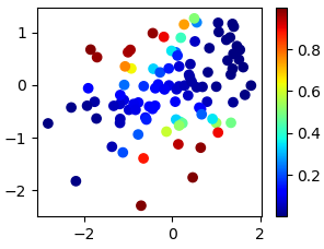
As one can see here, points on the top left and points on the bottom right are classified as musicals, but points in the area between are classified as not being musicals. This means that the region describing the “musical” concept is not convex or star-shaped – it is not even connected! This is certainly not what we want, because how would you define a prototypical point in this case?
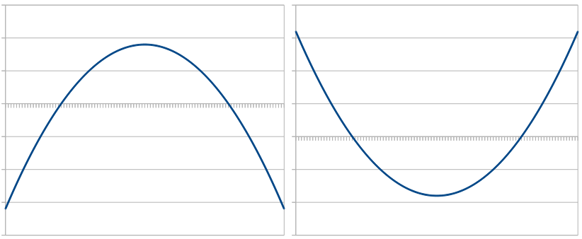
Remember that the inner term of the LTN membership function is a quadratic function, so it has the shape of a parabola. As illustrated in Figure 2, this parabola can either have a global maximum (left parabola) or a global minimum (right parabola). As stated above, the tanh() and the σ() functions take care of mapping the output of this quadratic function onto the interval [0,1] – the larger the value returned by the quadratic function, the higher the membership. If our network ends up producing a parabola like in the right part of Figure 2, then we get high membership values on the left and on the right side, but low membership values in the middle. This is exactly what happened in Figure 1. But what we actually want is a parabola like in the left part of Figure 2.
A convex variant
Luckily, there is a relatively simple trick to ensure that our parabola always looks like in the left part of Figure 2: We simply need to make sure that the coefficient a in y = ax2 + bx + c is negative. Because x2 is always positive, this ensures that for large absolute values of x the output of the function becomes very negative. Therefore, the quadratic function cannot have a global minimum, but only a global maximum – our parabola looks like the one in the left part of Figure 2.
This approach also generalizes to a higher number of dimensions – we then need to ensure that the weight matrix W in the formula for the membership function is negative semidefinite.
We can make any matrix A positive semidefinite by multiplying it with its transpose, and we can transform any positive semidefinite matrix into a negative semidefinite one by multiplying every entry with -1:
![]()
If we insert this into the original term, we get:
![]()
As you can see, we basically multiply Av with itself (which can only give us a positive result), and then multiply everything by -1. Analogously to ax2, we ensured that for larger absolute values of v, the output of the quadratic function becomes very negative. Again, this means that our parabola looks like in the left part of Figure 2 and that our membership function thus only has a single “peak” – which is exactly what we want.
The proposed modification is actually a quite small one – you only need to change a single line of code. But it guarantees that you always get convex regions out of an LTN.
In addition to this modification, I have also implemented three new membership functions, one of which is based on my formalization of conceptual spaces. I will talk about these further extensions of the LTN framework in a future blog post.
References
[1] Luciano Serafini and Artur d’Avila Garcez: “Logic Tensor Networks: Deep Learning and Logical Reasoning from Data and Knowledge” arXiv 2016. Link
hi, isn’t tanh(x) mapped onto the interval [-1,1] ? the [0,1] ones is sigmoid?
Yes, that’s correct. Looks like I’ve been a bit sloppy in my writing. What I meant is that you take the quadratic function, put it through the tanh (which maps to [-1,1]), then do another linear combination, and put the result of that through the sigmoid. What you get in the end is a result in [0,1], which is based on the quadratic function through the transformation with both tanh and sigmoid. Hope that makes things clearer. Thanks for pointing out that my explanation was not clear!