As stated earlier, the goal of my PhD research is to develop a system that can autonomously learn useful concepts purely from perceptual input. For instance, the system should be able to learn the concepts of apple, banana, and pear, just by observing images of fruits and by noting commonalities and differences among these images.
So far, I have mainly been talking about the conceptual spaces framework and how we can mathematically formalize it. However, as I want to actually end up with a running system, I need to implement my formalization in a computer program. So in today’s blog post, I’d like to introduce my implementation, which is publicly available: https://github.com/lbechberger/ConceptualSpaces
I’ve implemented my formalization using the programming language Python 2.7. I won’t go into too much detail with respect to how exactly everything was implemented. If you’re interested in that, please feel free to look at the code and/or my paper about this implementation [1].

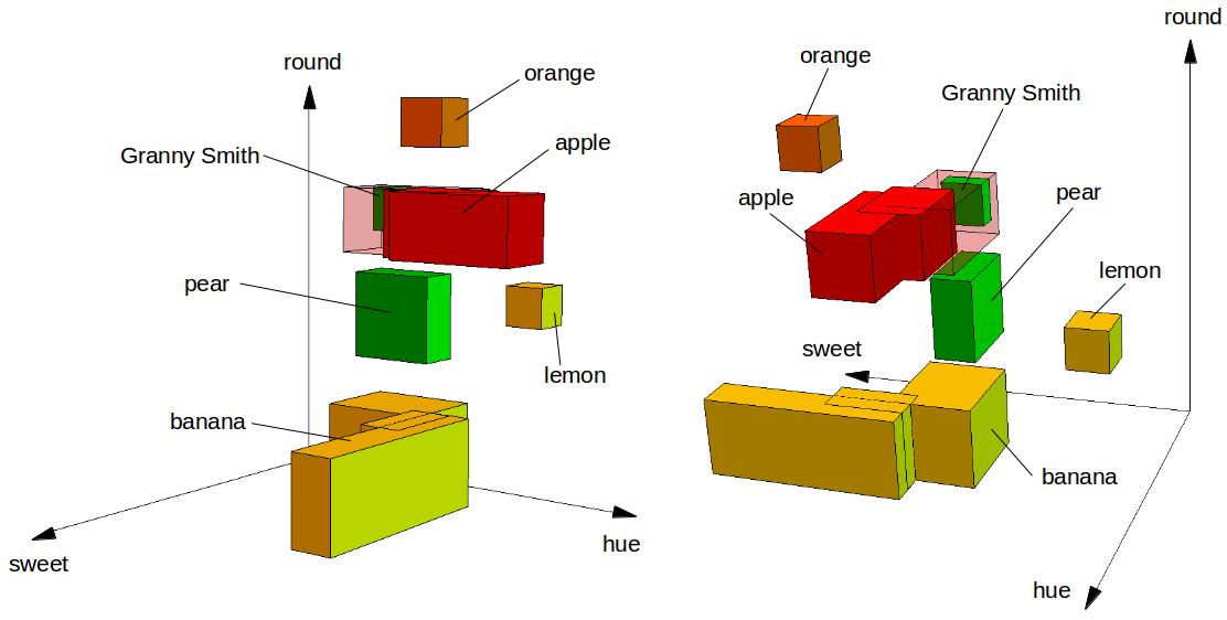
Instead of talking about implementational details, I’d like to give you a short illustration of how this implementation can be used. The GitHub repository contains a file called fruit_space.py which contains a simple conceptual space for fruits. You can imagine this space to look like in Figure 1. In the code, the space itself is defined as follows:
import cs.cs as space
domains = {"color":[0], "shape":[1], "taste":[2]}
dimension_names = ["hue", "round", "sweet"]
space.init(3, domains, dimension_names)
We define three domains (color, shape, and taste), each with a single dimension (namely: hue, round, and sweet). The concepts illustrated in Figure 1 are created as follows:
c_pear = Cuboid([0.5, 0.4, 0.35], [0.7, 0.6, 0.45], domains)
s_pear = Core([c_pear], domains)
w_dim = {"color":{0:1}, "shape":{1:1}, "taste":{2:1}}
w_pear = Weights({"color":0.50, "shape":1.25, "taste":1.25}, w_dim)
pear = Concept(s_pear, 1.0, 12.0, w_pear)
We first define the cuboid needed for the pear concept. That is, we define the box illustrated in Figure 1 by providing the coordinates of its corner points.
In the second line, we say that this cuboid constitutes the core of the “pear” concepts. One can also use multiple cuboids to define a core (which is for example done for the “banana” concept as you can see in the illustration).
The next two lines specify the weights for the different dimensions and domains. These weights reflect how important the different dimensions and domains are to the concept we are currently defining. In this example, both the shape and the taste domain are more important for the pear concept than the color domain. There are also other fruits that can be green (for instance bananas and apples), so shape and taste are more useful than color for figuring out whether something is a pear.
Finally, in the last row, we create a concept based on the core (s_pear) and these weights. The two additional numbers given in the definition of the concept are the maximal possible membership (1.0) as well as a sensitivity parameter (12.0) that controls the fuzziness of the concept (i.e., it determines the relationship between the distance of a point to the core and its membership value). If you want to understand in more detail what these numbers exactly mean, please refer to the paper about my formalization [2].
After having defined a number of concepts like this, we can use different operations on them, for instance the following ones:
pear.membership_of([0.6, 0.5, 0.4])
    1.0
pear.membership_of([0.3, 0.2, 0.1])
    0.0003526621646282561
print pear.intersect_with(apple)
    core: {[0.5, 0.625, 0.35]-[0.7, 0.625, 0.45]}
    mu: 0.6872892788
    c: 10.0
    weights: <{'color': 0.5, 'taste': 1.125, 'shape': 1.375},{'color': {0: 1.0}, 'taste': {2: 1.0}, 'shape': {1: 1.0}}>
In the first line, we ask to what extent the observation described by the coordinates [0.6, 0.5, 0.4] can be considered to be a pear. As these coordinates are within the cuboid we defined above, we get a result of 1.0 (i.e., 100% or full membership). For the point [0.3, 0.2, 0.1], which lies clearly outside of pear’s core, we only get a membership of about 0.00035 (i.e., 0.035% or very low membership).
We can also intersect the two concepts “pear” and “apple” (e.g., to get a conceptual description for things that we would consider to be both an apple and a pear to some extent). The output shown above is the definition of the resulting concept. However, these numbers don’t necessarily tell us too much – it’s sometimes hard to interpret them just by looking at them.
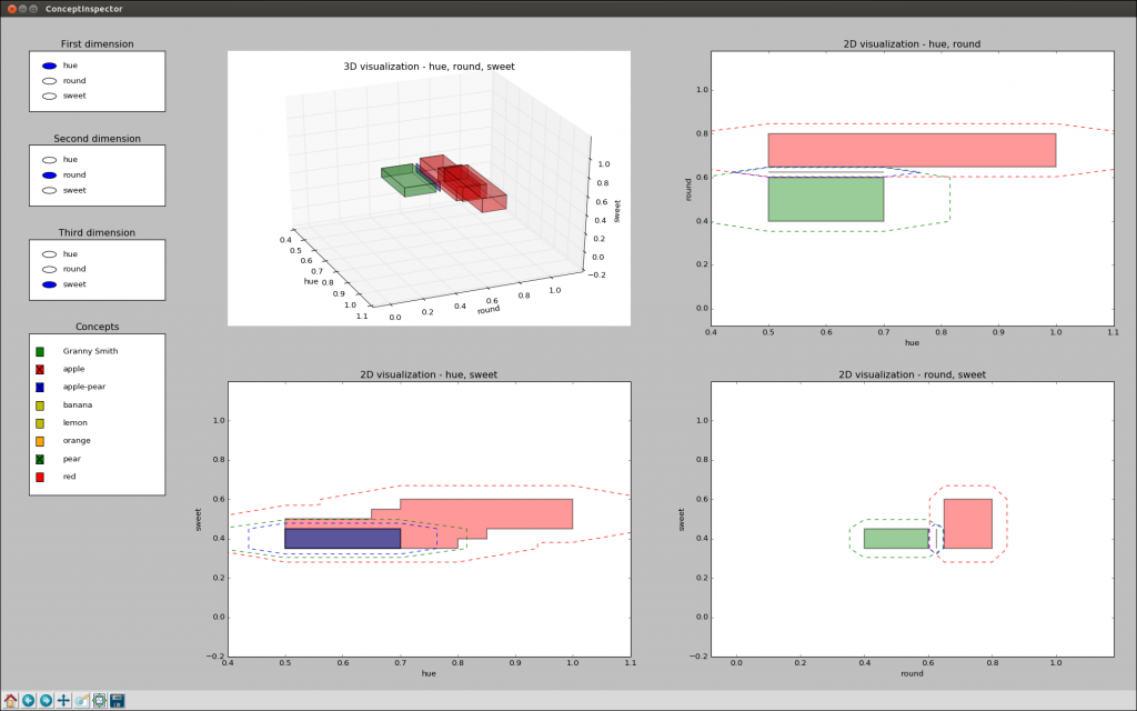
Fortunately, the implementation contains also a tool called the “ConceptInspector” which provides us with an interactive visualization of the conceptual space we are working with. This looks roughly as follows:

In the top left plot, we see a 3D visualization of all cores (similar to the one in Figure 1) that can be interactively rotated and zoomed. All other plots show the 2D projections of the cores as well as the 0.5-cuts of the sets. The radio buttons and check boxes on the left side of the window allow us to change the order of the dimensions and the concepts to be displayed, respectively.
As we can see in Figure 2 when looking closely, our new concept “apple-pear” (shown in blue) is between the concepts of “apple”(shown in red) and “pear” (shown in green), which makes intutive sense.
There are of course many more operations that you can use on the concepts, but I think this already suffices as a short introduction. If you are interested, a more thorough tutorial can be found on GitHub.
References
[1] Bechberger, Lucas and Kühnberger, Kai-Uwe. “A General-Purpose Implementation of Conceptual Spaces” under review for 5th International Workshop on Artificial Intelligence and Cognition. Preprint on arXiv.
[2] Bechberger, Lucas and Kühnberger, Kai-Uwe. “A Thorough Formalization of Conceptual Spaces” 40th German Conference on Artificial Intelligence, 2017.
