
I have already talked about multidimensional scaling (MDS) some time ago. Back then, I only gave a rough idea about what MDS does, but I didn’t really talk much about how MDS arrives at a solution. Today, I want to follow up on this and give you some intuition about what happens behind the scenes.
The overall job for an MDS algorithm is the following one: Given a number of dissimilarity ratings δij for pairs of items i and j and given a desired number t of dimensions, find for each item a point in a t-dimensional space such that the distances between two points accurately reflect the similarity rating of their underlying items.
One can typically distinguish two types of MDS algorithms (see, e.g. [1]):
“Classical” or “metric”‘ MDS assumes that the input values can be thought of as metric distances and that the differences and ratios of the similarity ratings are therefore meaningful. This is what I implicitly assumed in my previous post on MDS. For instance, if the item pair (A,B) has a similarity rating of 4, whereas the item pair (C,D) has a similarity rating of 2, then classical MDS assumes that the distance between the points representing C and D must be twice as large as the distance between the points representing A and B.
“Nonmetric” MDS on the other hand makes a much weaker assumption by only being concerned with the order of similarity ratings. In the example from above, nonmetric MDS only assumes that the distance between C and D must be larger than the distance between A and B. It however does not care about how much larger it is.
The dissimilarity ratings for pairs of items are typically acquired through psychological experiments. For instance, one can ask participants to rate the dissimilarity of two items on a 5-point scale from 1 (very similar) to 5 (very dissimilar). Because the ratings obtained from humans in such a way are quite noisy, one typically prefers to make as little assumptions as possible about them. Therefore, nonmetric MDS is preferred because it only assumes that the order of the dissimilarity values is meaningful, which is a relatively weak assumption. Metric MDS on the other hand also assumes that the differences and ratios of dissimilarity values are meaningful, which is a much stronger assumption that might not be valid.
I therefore focus on nonmetric MDS for the remainder of this blog post.
The first thorough mathematical treatment of the nonmetric MDS problem (along with a concrete algorithm for solving it) was given by Kruskal [2,3] in 1964. Although more efficient algorithms have been proposed since then, his papers lay out the overall idea of nonmetric MDS quite nicely. In this blog post, I will stay on a relatively high level of abstraction, but if you are interested in the mathematical details (which are not too complicated), I can definitely recommend looking at his papers.
Kruskal formulates the MDS problem as an optimization problem: The configuration of points in the t-dimensional space are varied in order to minimize a so called “stress” function. This stress function measures how well the current configuration of points reflects the dissimilarity values.
The stress value for a given configuration of points can be computed as follows: You sort all your dissimilarity values in ascending order, ending up with an ordering as shown in the next line:
δij< δkl < δmn < …
Now you compute the pairwise distances between the points representing the items i and j, k and l, etc. and you order these distances according to the ordering of the dissimilarity values:
[dij, dkl, dmn, …]
The stress function now basically checks whether this list is also in an ascending order (i.e., whether dij < dkl < dmn < …). If this is the case, the stress value is zero. If not, then it measures how much the distance values would need to change in order to achieve such an ascending order. Clearly, a small stress value is preferable.
The goal of the nonmetric MDS algorithm is now to find a configuration of points that minimizes this stress function. Kruskal proposes to use a gradient descent algorithm for this optimization. Let me illustrate gradient descent by an example:
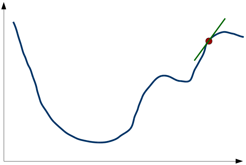
The x-axis of Figure 1 represents the variable that can be changed by the algorithm (in our case the coordinates of the points in the MDS space) and the y-axis represents the stress value. The blue line illustrates the stress function (which maps configurations of points to stress values). Given the current configuration of points, we can calculate the current stress value (illustrated by the red point). The gradient descent algorithm now also calculates the derivative of the stress function with respect to the configuration of points (the so called “gradient”). This is illustrated by the green line. In order to find the minimum of the stress function, the the configuration of points is changed in such a way that the value of the stress function decreases. In our example, this means that we have to move towards the left, because the derivative is positive. The gradient descent algorithm now makes a small step in this direction and ends up with a new configuration of points. Now we can again calculate the stress value, the derivative of the stress function and make another step in the direction where stress decreases. If we continue doing this, we will sooner or later end up in a point where the derivative is zero, i.e., in a “valley” of the stress function.
As Kruskal notes, this algorithm is always able to find such a valley (i.e., a local minimum), but we have no guarantee that we have found the deepest valley overall (i.e., a global minimum). For instance, in Figure 1 we might end up in the small valley to the right of the big valley. As you can see the stress value there is considerably higher. Knowing that there exists a much better solution, we’re therefore not happy with this local minimum. In order to solve this problem of local minima, Kruskal proposes to simply run the gradient descent algorithm multiple times, starting from different randomly chosen initial configurations. In our example, we will end up in the local minimum only if we start our journey in the right part of the diagram – if we start in the left part, we find the global minimum. By running the algorithm multiple times with different starting points, we have a fairly good chance of finding the global minimum at some point.
Once we have found a minimum of the stress function that we are happy with, the configuration of points that achieves this minimum is the solution of our MDS problem: This configuration of points is the one that reflects the dissimilarity values as faithfully as possible.
There are of course more efficient algorithms for MDS available these days and there is much more one can say about MDS (concerning for example missing dissimilarity values or ways to figure out how many dimensions are needed). I hope that for now the overall workings of nonmetric MDS have become reasonably clear. As mentioned before: If you are interested in mathematical details, please take a look at Kruskal’s papers.
References
[1] Wickelmaier, F. “An Introduction to MDS”. Sound Quality Research Unit, Aalborg University, Denmark, Citeseer, 2003, 46
[2] Kruskal, J. B. “Multidimensional Scaling by Optimizing Goodness of Fit to a Nonmetric Hypothesis”. Psychometrika, 1964, 29, 1-27
[3] Kruskal, J. B. “Nonmetric Multidimensional Scaling: A Numerical Method”. Psychometrika, 1964, 29, 115-129