
In my last blog post, I analyzed the differences of metric vs. nonmetric MDS when applied to the NOUN data base. Today, I want to continue with showing some machine learning results, updating the ones from our 2018 AIC paper (see these two blog posts: part 1 and part 2).
Overall Setup
In the experiments I report below, our regression target will always be the four-dimensional similarity space from Horst & Hout [1] who used metric MDS.
Overall, we consider a regression problem: For each image, we try to predict the coordinates of the corresponding point in the similarity space. As we have only 64 images in our data set, I used data augmentation in order to enlarge the number of training examples: For each original image, I created 1,000 distorted versions by adding noise, rotating, shrinking, zooming, and so on. At the end, we arrive at a data set with 64,000 images – a more reasonable size for applying machine learning. All distorted images based on the same original image are mapped onto the same point in the similarity space.
For evaluating how well the regression works, I make use of the coefficient of determination R². One can think of it as the percentage of variance in the ground truth targets that is being explained by the predictions of a regressor. In general, larger values are better.
For all experiments, I employed an eight-fold cross-validation scheme: I partitioned the overall data set into eight equally sized parts (each containing the augmented versions of eight original images). Then I used seven of these parts for training a linear regression (which estimates a linear model of the type y = mx + c) and the remaining part for evaluating the predictions of the model. By “rotating” this training-test split over the data set (such that each part is used for testing once) and averaging across all eight runs, I get the final evaluation results.
Question 1: How does the feature space affect the results?
In machine learning, having the right features for the task is often very crucial. I therefore compared two feature spaces in order to see which type of features is more useful for our regression task.
On the one hand, I used the high-level activations of the pretrained inception-v3 network [2] as a 2048-dimensional feature vector. On the other hand, I downscaled the augmented images from 300 x 300 to 25 x 25 pixels. Interpreting each color channel for each of these 625 pixels as a single feature results in a 1875-dimensional feature space. Both feature spaces are of comparable size, so any differences we may observe cannot be only explained by the number of features.
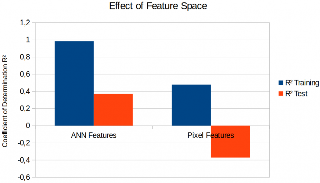
Figure 1 shows the results of a linear regression for both feature spaces. In both cases, performance on the training set is much better than on the test set, indicating that we have overfitting issues: Especially for the ANN-based features, it seems that the regression can almost perfectly memorize the training examples, but that it fails to generalize well to unseen examples in the test set.
Moreover, we see that the pixel-based features yield a negative value for R² on the test set – which means that the predictions of our linear model is actually worse than if we had always predicted a constant point (which would result in R² = 0). It thus seems that the ANN-based features are much more useful than the pixel-based features. One possible explanation is that the inception-v3 network extracts more abstract features than our surface-level manipulation of pixels, and that our task requires access to abstract rather than surface-level information. For the remainder of this blog post, we will stick with the ANN-based features.
Question 2: Does the structure of the similarity space support generalization to unseen examples?
The main idea of psychological similarity spaces is that they contain a meaningful structure: Similar items are closer to each other than dissimilar items. This meaningful arrangement of points in the similarity space should make it possible to generalize to unseen examples as visually similar inputs are mapped to close-by points. On the other hand, if the points in the similarity space were arranged randomly, even humans would have a hard time guessing where one should put a previously unseen item – visual similarity would not be helpful for making predictions.
In order to see whether this intuition is true, I have also shuffled the assignment of images to points in the similarity space and have trained a linear regression on these shuffled targets. Shuffling the target points destroys the semantic structure of the space, but it keeps the distribution of points in the space fixed. Figure 2 shows the results of this procedure.
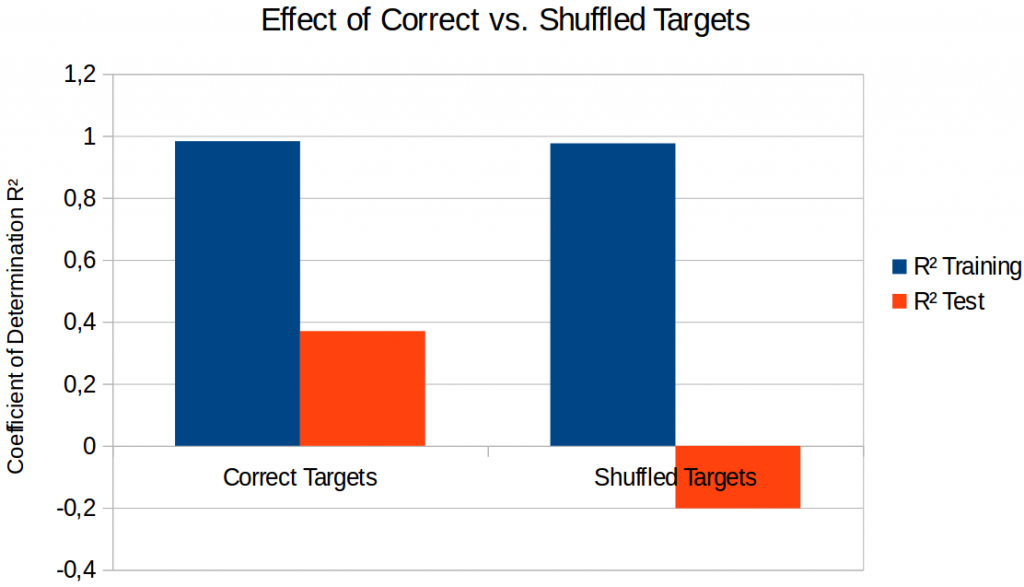
As we can see, training works comparably well in both cases. However, using a similarity space with a meaningful structure seems to be necessary in order to generalize to unseen inputs: If we shuffle the assignment of images to points (“Shuffled Targets”), the predictions on the test sets are again worse than a simple baseline that predicts a constant point. Overall, our intuition therefore seems to be true.
Question 3: Can we counteract overfitting by introducing regularization?
As seen before, the gap between training set performance and test set performance is quite large. We would like to reduce this gap by decreasing training set performance and increasing test set performance.
As we have 2,048 features and 4 output dimensions, the linear model contains 8,192 weights and 4 intercepts – quite a large number of parameters given that we have only 64 different target points in the similarity space. If a model has a large number of parameters to be estimated and if the data set is relatively small, one often observes overfitting tendencies: The regressor can easily find a configuration for these 8,196 parameters that works almost perfectly on the training set. However, this configuration of parameters might work only on this training set and not generalize well to other inputs. Instead of finding the perfect parameters on the training set, we should therefore look for reasonably good parameters – those might have a higher chance to work also reasonably well on other inputs.
The linear regression we have used so far estimates its parameters using a least-squares approach: It minimizes the squared difference between the model’s predictions and the actual ground truth. By introducing an additional regularization term that punishes large values of the model’s parameters, one obtains a so-called “lasso regressor”. If the strength of the regularization is set correctly, this can often help to reduce overfitting.
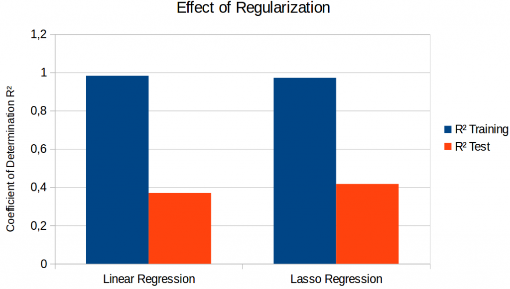
Figure 3 shows what happens if we introduce regularization. Although we are able to improve test set performance, we still have a very large gap between training and test set results: We are not able to get rid of the overfitting, we can only slightly reduce it.
It seems that the overfitting problem is part of our setup: After all, we have only 64 different target coordinates for estimating more than 8,000 parameters. The data augmentation helps to provide a larger number of slightly different feature vectors, but it is more of a crutch than an actual solution to the problem. Fighting overfitting seems to be the most important task for future work.
Summary & Outlook
So what have we learned today?
Overall, the approach seems to work reasonably well. “Deep” ANN-based features are more useful for our task than pixel-based surface-level information and the semantic structure of the similarity space seems to be necessary in order to achieve meaningful results. Even after introducing a regularization term, we still observe lots of overfitting, which gives us something to work on in the future.
In addition to the experiments reported above, I have also conducted experiments where I vary the target space for the regression (metric vs. nonmetric MDS and different number of dimensions). I will cover these additional results in my next blog post.
References
[1] Horst, J. S. & Hout, M. C.: “The Novel Object and Unusual Name (NOUN) Database: A Collection of Novel Images for Use in Experimental Research” Behavior Research Methods, 2016, 48, 1393-1409.
[2] Szegedy, C.; Vanhoucke, V.; Ioffe, S.; Shlens, J. & Wojna, Z.: “Rethinking the Inception Architecture for Computer Vision” Proceedings of the IEEE Conference on Computer Vision and Pattern Recognition, 2016, 2818-2826.
One thought on “A Hybrid Way: Reloaded (Part 2)”