
Some time ago, I wrote two blog posts about a hybrid way for obtaining the dimensions of a conceptual space (see here and here). Currently, I’m rerunning these experiments in a more detailed way and today I want to share both the motivation for doing this as well as some first results.
Motivation
Why do we have to re-do the experiments? Well, when I was reading about the underlying algorithms of multidimensional scaling (MDS), I noticed that there are two different types of algorithms: metric MDS and nonmetric MDS.
Metric MDS assumes that the dissimilarity ratings are ratio scaled. If the dissimilarity score of A and B equals 2 and the one between C and D equals 4, then metric MDS tries to arrange the points in the similarity space in such a way that C is twice as far away from D as A is from B.
Nonmetric MDS on the other hand assumes that the dissimilarity ratings are only ordinally scaled. In the example from above, nonmetric MDS would only try to arrange the points in the similarity space in such a way that A and B are closer together than C and D. The actual differences and ratios of the numeric distance values are not of interest in this case.
Okay, but so what?
Well, whenever you are dealing with dissimilarity ratings from psychological experiments, you want to make as little assumptions as possible about them. Therefore, the common recommendation is to use nonmetric MDS for dissimilarity ratings from psychological experiments. However, Horst and Hout [1] applied metric MDS to their NOUN data set – and so did we in our study [2]. But shouldn’t we have used nonmetric MDS instead?
Horst and Hout have elicited their similarity ratings with the SpAM approach [3], where participants are asked to arrange a set of stimuli on a computer screen in such a way that similar items are close together and that dissimilar items are far apart. They argue that one can use metric MDS in this case, because the dissimilarites have been measured as Euclidean distances between the items on the computer screen. However, one could argue that the participants might have only created a rough arrangement without paying too much attention to differences and ratios of distances. So maybe we should rather stick with the safe variant of nonmetric MDS.
I investigated this problem by simply running both MDS variants and by comparing their results. More specifically, the results shown in this blog post were derived based on the SMACOF algorithm implemented in the smacof library for R.
Looking at Stress
Remember that MDS tries to minimize a so-called “stress function”. This stress function measures the degree to which the current arrangement of points violates the information from the dissimilarity ratings. In nonmetric MDS, this stress function only checks whether the ordering of distances is correct, whereas in metric MDS, the stress function also takes into account the exact numerical values of the distances and dissimilarities.
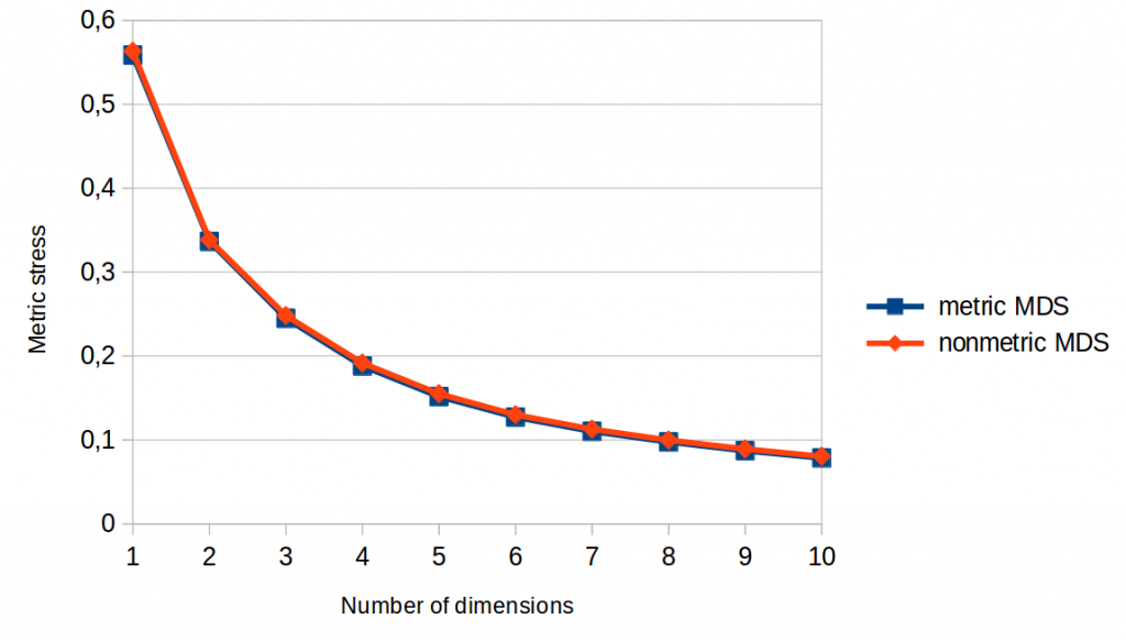
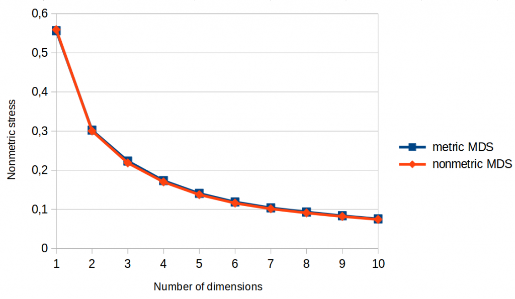
Figures 1 and 2 show so-called “Scree plots” which visualize stress as a function of the number of dimensions the MDS algorithm is allowed to use. In both graphs, we can see that the lines for metric and nonmetric MDS are pretty much identical.
As metric MDS makes use of more information than nonmetric MDS, and as metric stress is stricter than nonmetric stress, we would have expected that metric MDS performs better than nonmetric MDS with respect to the metric stress function (Figure 1): After all, metric stress evaluates the space based on information that only metric MDS had while creating the space. Nonmetric MDS on the other hand does not take the actual distance values into account when constructing the space (only their ordering), so we can’t expect it to get ratios and differences right.
However, this is exactly what we observe: Nonmetric MDS is just as good as metric MDS when it comes to metric stress, i.e., to making the numerical values of the distances align well with the numerical values of the dissimilarity judgments.
Long story short: According to Figures 1 and 2, using metric instead of nonmetric MDS does not seem to have any advantage.
Moreover, we can see in both Scree plots that stress seems to level off after five or six dimensions – hence we can assume that adding more dimensions will not be very beneficial. Moreover, using only a single dimension seems to be clearly not enough for a satisfactory solution.
Looking at Correlations
I further analyzed the correlation between the distances in the similarity space and the original dissimilarity ratings. Among others, I used Pearson’s correlation coefficient (which checks for a linear relation between two variables) and Spearman’s rank correlation coefficient (which only checks for a monotone relation).
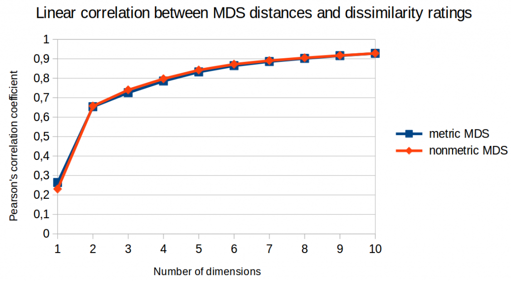
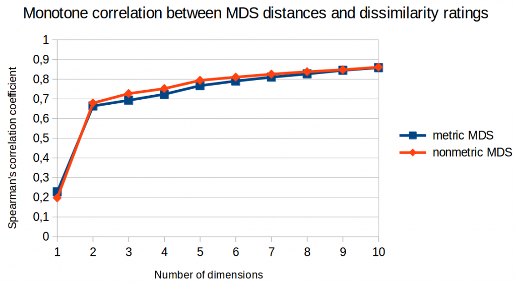
Figures 3 and 4 illustrate the results of this analysis. Again, we cannot see that metric MDS performs any better than nonmetric MDS. For Spearman’s rank correlation coefficient, we could even say that nonmetric MDS seems to perform slightly better.
So again: No advantage for metric MDS.
Moreover, we can again observe that performance is much better for two dimensions than for one dimension and that it saturates after five or six dimensions.
Looking at 2D Spaces
Finally, let’s take a look at the two-dimensional spaces generated by the two MDS variants. This visualization might be quite useful in order to see what’s going on.
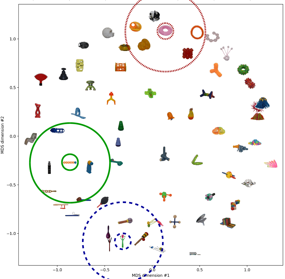
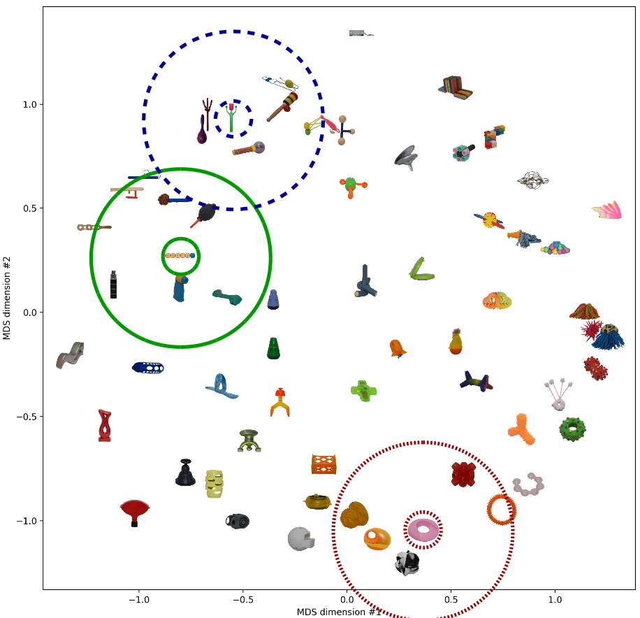
As we would expect based on the results from above, both spaces look quite similar. I have highlighted three objects and their respective neighborhood. These neighborhoods seem to make sense in both similarity spaces. Moreover, we note that in both spaces, the solid green neighborhood and the dashed blue neighborhood are quite close to each other while being relatively far away from the dotted red neighborhood. Also this seems to be a meaningful arrangement.
So also when looking at the resulting spaces, we see quite similar things.
Conclusion
Based on what I wrote above, there does not seem to be a big difference between metric and nonmetric MDS in our case (i.e., on this specific data set). As nonmetric MDS makes less assumptions about the underlying data, I would therefore recommend to always use nonmetric MDS when dealing with similarity data – using metric MDS only introduces additional assumptions, but does not necessarily improve your results.
In a next step, I want to rerun the machine learning part of the study, again comparing results for spaces from metric and from nonmetric MDS. Based on what I wrote today, I however expect no big differences between the two variants.
As we observed that using more than six dimensions does not seem to be very useful (both with respect to stress and with respect to correlation), I will focus on spaces with two to six dimensions.
Code for reproducing the results reported here can be found in my GitHub repository.
References
[1] Horst, J. S. & Hout, M. C.: “The Novel Object and Unusual Name (NOUN) Database: A Collection of Novel Images for Use in Experimental Research” Behavior Research Methods, 2016, 48, 1393-1409.
[2] Lucas Bechberger and Elektra Kypridemou: “Mapping Images to Psychological Similarity Spaces Using Neural Networks” AIC 2018.
[3] Goldstone, R.: “An Efficient Method for Obtaining Similarity Data” Behavior Research Methods, Instruments, & Computers, 1994, 26, 381-386
2 thoughts on “A Hybrid Way: Reloaded (Part 1)”