
Last time, we talked about the transfer learning results. Today, it’s time to take a look at the multi-task learning approach. Let’s get started.
Motivation
In the transfer learning setup considered last time, training consisted of two phases: We first trained the network on a classification task, and then trained a linear regression on top of its learned representation. This time, we’ll consider a multi-task learning setup where we learn the mapping and the classification at the same time.
What’s the theoretical advantage of multi-task over transfer learning? There are two aspects to consider: First of all, we have a better control over the trade-off between the two tasks. As mentioned earlier, we optimize a linear combination of the classification loss and the mapping loss. By varying the relative weight of these two losses, we can explicitly control how much emphasis is put on the respective tasks. In the transfer learning setting, on the other hand, we cannot explicitly control this trade-off, since we have two separate training phases that focus both to 100% on their respective task.
In our specific setup, multi-task learning has another advantage over transfer learning: Since we use a part of the bottleneck layer to represent the coordinates in our similarity space, the gradient coming from the classification output creates additional constraints on the output units for the mapping task. Since we have only a very limited number of distinct target coordinates, this may turn out to be very helpful, since it may prevent the output units of the mapping task from overfitting.
Methods
Okay, so how did I conduct the multi-task learning experiment? Well, I used three of the network configurations identified in the classification experiments, namely, Default, Small, and Correlation. I retrained them from scratch, using different strengths of emphasis on the mapping task, namely:
λ = 0.0625, 0.125, 0.25, 0.5, 1.0, 2.0
Here, a weight of λ = 0.25 reflects the proportion of examples for the mapping task in our augmented data set. A stronger emphasis may be useful, but also comes with an increased risk of overfitting. Hence, I test both larger and smaller values of λ.
Again, I use a five-fold cross validation and evaluate the mapping results based on MSE, MED, and R². I also consider classification accuracy on both TU Berlin and Sketchy, as well as the correlation of distances in the overall representation space to the original dissimilarity ratings from the psychological study. I compare the results with respect to all of these metrics to the results obtained by the transfer learning approach.
Results
So let’s take a look at the results. For the sake of simplicity, I’ll only focus on the coefficient of determination R² for the regression results. Both the MSE and the MED paint a similar picture, so I won’t present them here.
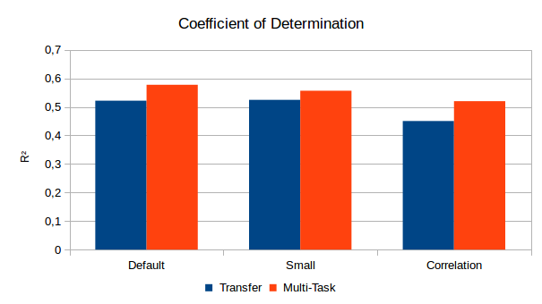
As we can see in Figure 1, the multi-task learning approach is able to considerably outperform the transfer learning approach with respect to all three configurations. The largest improvement can be observed for the Correlation configuration (for λ = 2.0). However, the results are still considerably worse than for other configurations. The best overall performance was obtained with the Default setup with R² ≈ 0.58 (using λ = 0.0625), followed closely by the Small configuration (λ = 0.125).
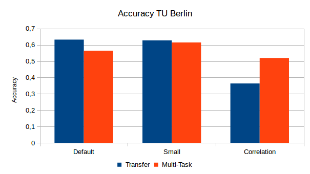
How much classification accuracy do we need to sacrifice in order to get the improved regression results? Figure 2 shows some interesting effects: Multi-task learning in the Default setting led to a considerable drop of classification performance (about 7 percentage points), while only a minor change (a bit more than 1 percentage point) was observed for the Small configuration. The Correlation configuration on the other hand manages to considerably improve classification accuracy in the multi-task setup.
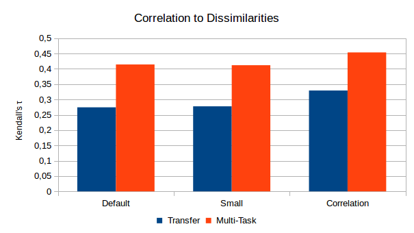
Finally, what about the correlation between distances in the representation space and the original dissimilarity ratings? Again, we see a clear improvement for all three configurations when using the multi-task learning approach. The Correlation configuration reaches the highest values with τ ≈0.45, but it also started from a higher level in the transfer learning condition. Moreover, both the Default setup and the Small configuration achieved similar levels of correlation if a large mapping weight of λ = 1.0 or λ = 2.0 was used.
Discussion
So what do these results mean?
Joint training of both the classification and the mapping task seems to be helpful. This may be based both on the ability to fine-tune the trade-off between the two tasks and on the additional constraints for the mapping output coming from the subsequent classification layer. Investing more effort into a more complex setup thus seems to have payed off. Overall, small values of λ seem to be preferable, indicating that we have to worry about overfitting in the mapping task.
The sacrifices made for an improved mapping performance are negligible for the Small configuration (where we have only 256 units in the bottleneck layer), but notable for the Default configuration (which uses 512 bottleneck units). This is somewhat surprising, since the two configurations differ only with respect to the size of their bottleneck layer: One would expect that a larger number of units allows for more redundancy and thus more “slack” to cope with additional constraints. In our experiments, the opposite seems to be true. This urges for further investigations.
With respect to the Correlation configuration, it seems that the mapping task proved to be a valuable way of regularization for the classification task: Having to predict also correct coordinates in shape space prevents the network from overfitting the training set with respect to making classifications. The mapping task thus acts as a reasonable substitute for dropout, which had been disabled in this configuration. This is also supported by the large emphasis (λ = 2.0) put on the mapping task.
The increase in the correlation to the dissimilarities does not come as a big surprise: After all, we try to align part of the network’s representation with the shape similarity space that has been explicitly based on these dissimilarity ratings. Success in the mapping task thus also implies an increased level of correlation.
Outlook
Overall, our results are still reasonably poor: A coefficient of determination of R² ≈ 0.57 is still considerably too low for practical applications. So we may need to step up our game even further to achieve even better results. The number of distinct data points in the shape space (in our case 60) may however put a hard limit on the performance level one can obtain in practice. I therefore leave further performance improvements to future work.
Instead, I will take a look at the generalization capability of our two setups (transfer learning and multi-task learning) to target spaces of different dimensionality. This will probably be the topic of the next blog post in this little series.
Another line of experiments waiting to be conducted concerns the use of an autoencoder rather than a classification network: Instead of predicting sketch classes, we can train an autoencoder to reconstruct the images from a compressed hidden representation. Maybe this reconstruction objective is closer to the perceptual level and leads to more promising results. I’ve currently started the first set of experiments in this direction. However, since this setup requires training two networks instead of one, and since the number of output units (and hence sources for the gradient update) is much larger, computation is veeery slow. I’ll definitely write a blog post on those results, but it may take a while until I have some first numbers to share.