
It has been over a year since my last blog post and I have left with something like a cliff hanger: The results from the last set of machine learning experiments with the autoencoder (see also here and here) were still missing. Now that I have finally handed in my dissertation, I am able to finish this already quite long series of blog posts. So let’s recap what still needs to be investigated…
Experimental Setup
Please recall, that last time, I reported results on both transfer learning and multi-task learning for the autoencoder approach. We observed, that the autoencoder yielded much weaker results than what we had seen for the classifier network in earlier blog posts (here and here). This was somewhat disappointing, given the increased training cost for an autoencoder with its more complex loss function and its additional decoder network.
In analogy to the generalization experiments for the classifier-based network, I now report on the final set of experiments, where the best autoencoder setup from the 4-dimensional target space was retrained (without further hyperparameter optimization) on target spaces from 1 to 10 dimensions. For the reconstruction-based transfer learning approach, I used a lasso regression with β = 0.02, while for the multi-task learner, I used a relative weight of the mapping task of λ = 0.0625. These two values had led to the optimal performance reported in the experiments from last time, both being based on the best configuration of hyperparameters.
Results and Interpretation
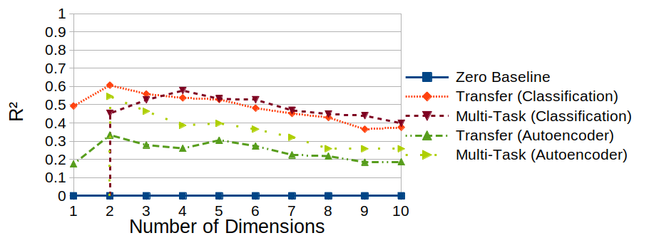
Figure 1 shows the results from these experiments (for the sake of simplicity, only considering the coefficient of determination R²), also in comparison to the classfication-based results. What can we observe?
Well, first of all, the autoencoder performs consistently worse than the classifier in pretty much all target spaces, confirming what we had observed last time. There, we also speculated, why this may be the case – namely, because the autoencoder needs to encode small details (like the exact size and location of the object in the picture), from which the classifier can abstract away. The only glimpse of hope is the two-dimensional target space, where the reconstruction-based multi-task learner outperforms its classifier-based counterpart.
When taking a closer look at the generalization pattern across the target spaces, we can spot a difference between classifier-based and reconstruction-based approaches: For the autoencoder, both learning setups reach their peak performance for the two-dimensional space. For the classifier, the multi-task learner performed best in a four-dimensional target space, while the transfer learning approach worked best in a two-dimensional space. Moreover, for the autoencoder, the two curves seem to run almost in parallel (with multi-task learning consistently outperforming transfer learning), while no such clear picture emerges for the classifier-based approach.
So what does this tell us? Well, the bottom line seems to be, that the increased overhead of training an autoencoder does not pay off at all, but that reconstruction-based approaches seem to show a more predictable generalization behavior.
General Summary and Outlook
Okay, so this was the last set of experiments in my “Learning To Map Images Into Shape Space” series. What have we learned overall?
In general, multi-task learning seems to be preferable over transfer learning – here, the additional overhead of re-training the whole network pays off in the form of considerably improved performance. Moreover, classifiers seem to be a better starting point for the mapping task than autoencoders, since the reconstruction objective is somewhat in conflict with our data augmentation of resizing and relocating the object in the image.
Overall, the performance level is still way too low for any practical applications. However, the transfer learning experiments by Sanders and Nosofsky [1] on a larger dataset of 360 stimuli show, that more data can improve performance: They report a top value of R² ≈ 0.77, while my best setup only reached R² ≈ 0.61.
Finally, if you want to take a closer look at my setup and results, I can redirect you to the paper [2] (which has finally been officially published a couple of days ago) and to my GitHub repository.
Since I’ve now handed in my PhD and since I’m leaving academia for now, this will probably be the last entry on this blog, at least for a while. Thanks for reading! 🙂
References
[1] Sanders, C. A. & Nosofsky, R. M. Using Deep-Learning Representations of Complex Natural Stimuli as Input to Psychological Models of Classification Proceedings of the 2018 Conference of the Cognitive Science Society, Madison., 2018
[2] Bechberger, L. & Kühnberger, K.-U. Grounding Psychological Shape Space in Convolutional Neural Networks 3rd International Workshop on Cognition: Interdisciplinary Foundations, Models and Applications, 2021