
Today it’s finally time to look at the mapping results based on the autoencoder discussed last time. We’ll take a look at both transfer learning and multi-task learning, using the same overall setup as for the respective classification-based experiments described here and here.
Methods
For recontruction-based transfer learning, I used the pre-trained network configurations (called default and best) of the autoencoder (discussed here) and extracted the bottleneck activations for all images of the augmented data set. I then trained both a linear and a lasso regression from this feature space into the four-dimensional mean similarity space and evaluated the whole thing in a five-fold cross validation. Like in all prior experiments, I used 10% salt and pepper noise during training, but no noise during testing. The setup is thus pretty much identical to the one described for transfer learning based on the sketch classifier.
Also for multi-task learning, I considered again the default and best configurations of the autoencoder’s hyperparameters. I retrained the respective network from scratch using both the reconstruction objective (with a fixed weight of one) and the mapping objective (exploring the same possible mapping weights as for the classifier-based multi-task learning experiments). Again, I used a five-fold cross validation and 10% noise during training, but none during testing. The four-dimensional mean similarity space was again used as regression target.
Results
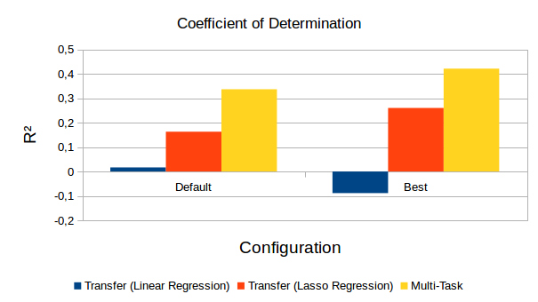
Figure 1 summarizes the results of these experiments using the coefficient of determination R² as evaluation metric. As we can see, the linear regression performs very poorly with a value of R² of slightly above or even below zero. This is pretty bad, because even a simple baseline that always predicts the origin of the coordinate system is able to achieve R² = 0! Using regularization in the form of a lasso regressor improves these results, but only to a very modest performance level of R² ≈ 0.17 and R² ≈ 0.26, respectively. If we use multi-task learning, we can furthermore improve our results up to R² ≈ 0.34 and R² ≈ 0.42. This is however still considerably worse than what we had observed for our classification-based experiments, where we obtained R² ≈ 0.52 in the transfer learning setting and R² ≈ 0.58 by using multi-task learning. Overall, the best configuration seems to yield better results than our default setting not only with respect to reconstruction quality (see here), but also with respect to mapping performance. We can thus conclude that the hyperparameter tuning has been worth the trouble.
But why do my autoencoders perform so poorly overall? As it turns out, the autoencoder does not only need to encode the overall shape of the depicted object in its bottleneck layer, but also the exact location and size of this object. This is necessary in order to accurately reconstruct the original image. It seems that shape-related information is not stored separately from size and location data, but all of them are mashed together in a tightly entangled representation. This means also that we cannot simply “read out” only the shape-related pieces of information from the bottleneck layer by using a linear or lasso regression.
A classifier on the other hand can choose to ignore the size and location information in its internal representation, since they are not needed for making the correct classification. We therefore don’t face these entanglement issues, since information about size and location of the object is largely discarded from the internal representation. It is thus much easier to access shape-related information for the mapping task.
Outlook
So it looks like using an autoencoder as starting point for my hybrid procedure does not pay off in terms of mapping performance, it only makes training much more computationally expensive, which is a bummer. Nevertheless, I want to conclude my experiments by also looking at the generalization to target spaces of different dimensionality in my upcoming blog post – which will then also mark the end of the quite long “Learning To Map Images Into Shape Space” series.