
As already mentioned last time, I’m currently running some mapping experiments with autoencoders. Today, I can share some first results of the raw reconstruction capability of the trained autoencoders.
Motivation
In my previous posts, I have considered transfer learning, multi-task learning, and a generalization to other target spaces for a classification-based encoder network. I’ve started with a classification task, since a comparison of classification performance to other classifiers from the literature is quite straightforward – I was thus able to judge whether my overall training setup was sound before looking at the mapping task itself.
But why should we now also take a look at an autoencoder? Basically, there are two motivations:
Firstly, the training signal for the autoencoder (namely, the difference between its reconstruction and the original input) is much closer to the raw perceptual level than a classification objective. Since we are interested in low-level shape perception, one may speculate that the features learned by an autoencoder are a better match to our shape spaces than the features learned by a sketch recognition network.
Secondly, the decoder network of the autoencoder provides us with a way of visualizing points in the similarity space. We can manipulate points in the shape space and then use the decoder network to visualize how these manipulation change the shape of the respective object. For instance, one can investigate linear interpolations between pairs of stimuli, or one can verify whether movements along the interpretable directions result in the expected changes in the image.
Based on these two motivations, it seems worthwhile to investigate also autoencoders with their reconstruction objective as a starting point for learning a mapping into similarity spaces. In today’s blog post, we’ll limit ourselves to training a plain autoencoder without considering the mapping task at all.
Methods
For the encoder network, we used the same structure as in our classification experiments (i.e., the Sketch-a-Net architecture [1]), such that any difference we observe can be attributed to the type of loss function being used (since this is the only major thing that has changed).
The overall structure of the decoder network has already been described in this old blog post. However, since I’m dealing with larger images (224 × 224 pixels instead of 128 × 128 pixels), the sizes of the individual layers have been slightly changed.
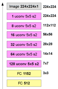
Figure 1 shows the updated structure of the decoder network. The main change to the previous version is that we use 1152 units in the second fully connected layer (corresponding to a 3 × 3 image with 128 channels) instead of 2048 (which corresponded to a 4 × 4 image with 128 channels) and that we added another upconvolutional layer to the hierarchy. In comparison to Dosovitskiy and Brox [2], we use thus one additional layer, but a smaller number of kernels in each layer and a smaller number of units in the fully connected layer. Overall, our decoder has 1.5 million trainable parameters.
We trained the network on augmented images from Sketchy and TU Berlin, as well as on our line drawings and a set of 70 additional line drawings from a related study. We used 10% salt and pepper noise on the inputs, but the autoencoder had to reconstruct the uncorrupted image. That is, we trained a denoising autoencoder [3]. Again, we used a five-fold cross validation and report averaged values across all folds.
The network was trained to minimize a binary cross-entropy loss between the image and its reconstruction. We again trained for 200 epochs and selected the iteration with optimal validation set performance for application to the test set.
Results
I explored the influence of different hyperparameters on the results by varying all of them individually, starting from a given default setting. I gained the following insights:
Removing the weight decay term from the encoder completely improved reconstruction performance over the default setting of 0.0005. Disabling dropout in the encoder was also beneficial.
Enabling dropout in the decoder turned out to worsen our results. Similar observations were made for the introduction of a weight decay penalty for the decoder.
Increasing the level of salt and pepper noise led to a slight to drastic reduction of both correlation and reconstruction performance. The reconstruction loss was quite robust with respect to different sizes of the bottleneck layer, but the correlation to the dissimilarities suffered for smaller bottleneck layer sizes.
Based on these insights, I conduced a small grid search, where I varied the size of the bottleneck layer (512 vs. 256 units) and the weight decay for the encoder (0 vs. 0.0005). All other regularization techniques (weight decay for the decoder as well as dropout) were deactivated and I used 10% salt and pepper noise. As it turns out, the best results were obtained by using a large bottleneck layer with disabled weight decay.

Figure 2 illustrates the reconstruction performance of the trained network: Figure 2a compares the original image (Image license CC BY-NC 4.0, source) to the reconstruction with the default setup and the best setup identified in the grid search. As we can see, the reconstruction performance improves considerably when optimizing the network’s hyperparameters. Figure 2b shows different reconstructions of the same original image for different random noise patterns and illustrates that our network successfully filters out noise. Figure 2c compares different levels of noise (0%, 10%, 25%, and 55%) – if there is considerably more noise in the image than expected by the network, reconstruction fails.
Outlook
The reconstructions obtained by our best hyperparameter configuration look promising – the overall shape of the object is quite well preserved and even some details (such as the form of the tail or the existence of a wing) are preserved. This means that the network is capable of representing shape-related information in its bottleneck layer, including information about our three psychological features FORM, LINES, and ORIENTATION.
In my next posts, I will use this learned representation both for a transfer learning task and in a multi-task learning scenario. Will good reconstructions allow us to make an accurate mapping? We’ll see next time…
References
[1] Yu, Q.; Yang, Y.; Liu, F.; Song, Y.-Z.; Xiang, T. & Hospedales, T. M. Sketch-a-Net: A Deep Neural Network that Beats Humans International Journal of Computer Vision, Springer, 2017, 122, 411-425
[2] Dosovitskiy, A. & Brox, T. Inverting Visual Representations With Convolutional Networks Proceedings of the IEEE Conference on Computer Vision and Pattern Recognition (CVPR), 2016
[3] Vincent, P.; Larochelle, H.; Bengio, Y. & Manzagol, P.-A. Extracting and Composing Robust Features With Denoising Autoencoders Proceedings of the 25th international conference on Machine learning – ICML ’08, Association for Computing Machinery (ACM), 2008
2 thoughts on “Learning To Map Images Into Shape Space (Part 8)”