After having spent already four (!) blog posts on the general and specific setup for my current machine learning study (data set, architecture, experimental setup, and sketch classification), it is now finally time to reveal the first results of the mapping task with respect to the shape domain. Today, we’ll focus on the transfer learning setup before looking into the multi-task learning results in one of the next posts.
Methods
In the transfer learning experiments, I extracted the high-level activations of pre-trained networks for all the augmented versions of the original line drawings. I then trained a linear regression and a lasso regression from these feature spaces into the four-dimensional Shape space from our Shapes study. The overall setup of these transfer learning experiments is thus pretty much identical to the ones of the NOUN study [1].
For evaluating the resulting mapping, I will focus on the coefficient of determination R², which tells us how much of the variance in the data can be explained by our model. For all feature spaces, I used a five-fold cross validation and only talk about averaged results here. I used 10% salt and pepper noise during training, but no noise for testing.
In the NOUN study, I had only used the inception-v3 network [2], which had been trained on photographs. In the current experiment, I also considered different variants of our sketch classification network, namely Default, Large, Small, and Correlation (as introduced in part 4 of this series). Comparing the two network types can tell us something about the importance of the source domain (photographs vs. sketches) for our target domain of line drawings.
Results

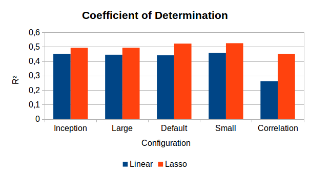
Figure 1 shows a bar chart of the main results. We can see that the linear regression performs comparably well across all configurations at a level of 0.44-0.46. The only notable exception is the Correlation configuration, where we only achieve a value of R² = 0.26. Using regularization in the form of a lasso regression helps to improve results in all cases. Here, our Default and Small configurations reach slightly, but consistently higher values than the Inception baseline and the Large configuration (both of which have 2048 dimensions). Reducing the size of the feature space thus seems to be helpful in counter-acting overfitting tendencies.
The Correlation configuration profits most from regularization, but this may be based on its poor performance in general: Even when using regularization, it is only able to reach the performance level that the other configurations had without regularization. It thus seems that the correlation to the dissimilarities is not a very useful predictor for selecting promising network configurations for the mapping task.
Discussion
The results from above contain some good news and some bad news for our overall research goal.
The good news is twofold: First of all, our sketch-based network gives better performance than an off-the-shelf pre-trained photo-based network. So all our efforts so far were not unnecessary and using sketches rather than photographs as a source domain does pay off. Secondly, the best results obtained with the Inception feature space (R² = 0.49) are considerably better than what analogous experiments on the NOUN data set had shown (where we obtained R² = 0.39 on a four-dimensional target space). Thus, focusing on a single cognitive domain seems to make things easier.
Also the bad news is twofold: On the one hand, the improvements over the Inception baseline is quite small – we go from R² = 0.49 to R² = 0.52. One may thus wonder whether training a network from scratch is really worth it (since this is quite time consuming). On the other hand, Sanders and Nosofsky [3] have reported much higher values of R² = 0.77 for a regression into an eight-dimensional similarity space. They used a larger data set and a more complex network architecture, which raises the question whether we also need to consider a more sophisticated setup.
Outlook
So although we have somewhat promising results, it is obvious that the current transfer learning setup is not the final answer. In the next blog post of this series, we will thus talk about the multi-task learning setup, where we learn the classification task and the mapping task at the same time, hoping for a nice performance boost.
References
[1] Bechberger, L. & Kühnberger, K.-U. “Generalizing Psychological Similarity Spaces to Unseen Stimuli” 2021.
[2] Szegedy, C.; Vanhoucke, V.; Ioffe, S.; Shlens, J. & Wojna, Z.: “Rethinking the Inception Architecture for Computer Vision” Proceedings of the IEEE Conference on Computer Vision and Pattern Recognition, 2016, 2818-2826
[3] Sanders, C. A. & Nosofsky, R. M. “Using Deep-Learning Representations of Complex Natural Stimuli as Input to Psychological Models of Classification” Proceedings of the 2018 Conference of the Cognitive Science Society, Madison., 2018

3 thoughts on “Learning To Map Images Into Shape Space (Part 5)”