
In one of my last blog posts, I have introduced a data set of shapes which I use to extract similarity spaces for the shape domain. As stated at the end of that blog post, I want to analyze these similarity spaces based on three predictions of the conceptual spaces framework: The representation of dissimilarities as distances, the presence of small, non-overlapping convex regions, and the presence of interpretable directions. Today, I will focus on the first of these predictions. More specifically, we will compute the correlation between distances in the MDS-spaces to the original dissimilarities and compare this to three baselines. This will help us to see how efficiently the similarity spaces represent shape similarity.
Before we take a look at the results of this analysis, let me introduce the three baselines in more detail.
The Pixel Baseline
The pixel baseline uses raw pixel information to compute a distance between two images. The idea of this baseline is that maybe the raw pixels already contain enough information to predict the shape similarity of two images. Since the information about individual pixels might be too fine-granular, I also consider more coarse-grained versions of the images by downscaling them (e.g., from 283×283 pixels to 10×10 pixels). These downscaled versions of the original images presumably only contain information about the rough shape of the object, but are unable to represent (potentially unnecessary) details any more.
More specifically, I divided the images into blocks of size k×k and computed the minimum across all values inside each block as a value for the overall block itself. Each image is then represented as a vector containing the values of its blocks and the distance between tow images is computed as a distance between their corresponding vectors. I tried all possible values for the block size k, but I only report the results for the best choice of k below.
The ANN Baseline
Artificial neural networks have achieved outstanding results in image classification tasks. Kubilius et al. [1] have argued that this is because these networks implicitly learn a model of the shape domain. The ANN baseline uses this assumption and represents each image by the high-level activation vector of a pre-trained neural network (more specifically, the inception-v3 network [2]). The distance between the images is then computed as the distance between these activation vectors.
Since deep learning models extract a nonlinear transformation of the input data, the ANN baseline thus assumes that raw pixel information is not enough for predicting shape similarities, but that such a complex nonlinear transformation is necessary. By using a pre-trained neural network, I furthermore assume that the relevant shape features are implicitly learned when doing image classification and that they can be easily transferred to our data set.
The Feature Baseline
Our third baseline makes use of the three features FORM, LINES, and ORIENTATION as introduced last time. Essentially, the feature baseline assumes that these three features are sufficient for describing the shapes of our data set. Thus, every image is represented by its rating with respect to the three features, resulting in a vector with three entries. The distance between two images is then calculated based on these feature vectors.
While both the pixel baseline and the ANN baseline operate on the images themselves, the feature baseline operates on psychological ratings. If the dissimilarity ratings can be explained by our three features, then the feature baseline should be as good as the MDS-based similarity spaces.
The General Procedure
Okay, so in total we have four competitors: Our similarity spaces (with a varying number of dimensions), the pixel baseline, the ANN baseline, and the feature baseline. All of these competitors represent an image by a feature vector and distances between images are represented by distances between these vectors. So far, I have however not specified how this distance between vectors is computed.
For each of the four competitors, I have tried using the Euclidean metric, the Manhattan metric, and the inner product as distance functions. While we expect that the Euclidean metric works best for the similarity spaces, it is less clear which distance function to use for the baselines. Below, I only report the best result for each competitor.
Peterson et al. [3] have observed that applying individual weights to the entries of an ANN’s activation vector can improve the predictions of psychological dissimilarities. This is quite related to the salience weights of the conceptual spaces framework. In order to take this into account, I have also optimized dimension weights for each of the distance functions used above. Again, I only report the best results below.
The Results
Okay, now it’s finally time to look at our results. The overall correlation between distances and dissimilarities has been measured with Kendall’s τ and is visualized in Figure 1. Let us take a look at the different competitors individually.
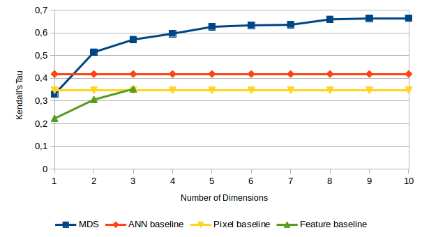
Let’s start with our MDS-based similarity spaces which have been obtained using nonmetric SMACOF. As we can see in Figure 1, adding more dimensions to the similarity space helps to improve the correlations. However, the curve flattens after five dimensions indicating that a five-dimensional similarity space is sufficient for our data set. The largest improvement happens between one and two dimensions. The best configuration for the MDS-based similarity space was the Euclidean distance without dimension weights. This is however not a surprise, since MDS explicitly arranges the points in such a way that their unweighted Euclidean distance reflects the dissimilarities as well as possible.
For the pixel baseline, the highest correlation was observed for a block size of k = 2 (i.e., still very detailed images of size 142×142, corresponding to 20,164-dimensional feature vectors), optimized weights, and the Euclidean distance. The correlations between these distances and the dissimilarities was however not considerably higher than the correlations achieved for a one-dimensional MDS space. We can therefore conclude that raw pixel information is not sufficient for predicting the dissimilarities from our data set.
As one can see in Figure 1, the ANN baseline (using a 2,048-dimensional feature vector) performs considerably better than the pixel baseline. This indicates that the nonlinear transformation of the raw pixel information is indeed helpful in our scenario. However, the ANN baseline is clearly outperformed already by a two-dimensional similarity space based on MDS. This can however at least partially be attributed to the fact that the network was trained on classifying photographs, while we apply it to predicting similarities between line drawings. On the other hand, one may be tempted to conclude that the features of the pre-trained network are not identical to the features used by humans when making similarity judgements. Also for the ANN baseline, the Euclidean distance with optimized dimension weights yielded the best results. In fact, here the weight optimization had by far the largest impact among all competitors.
In contrast to all other competitors, the Manhattan distance yielded the best results for the feature baseline. Using optimized dimension weights slightly improved performance, but did not yield considerable differences to an unweighted version of the distance metric. This indicates that all three features seem to be of similar importance. However, as we can see in Figure 1, the correlation of the distances predicted by the feature baseline to the actual dissimilarities is considerably lower than the correlations observed for the MDS solutions. This indicates that our three features FORM, LINES, and ORIENTATION are not sufficient for capturing all necessary nuances of shape similarity. However, if more features are included in the future, the gap between the feature baseline and the MDS spaces may be reduced.
And Now?
So what is the bottom line of these results? Obviously, spaces explicitly extracted from the dissimilarity ratings do a better job at reflecting these dissimilarity ratings than baselines which are based on other sources of information. This by itself is not an interesting result.
However, we can still learn something from this analysis: Since none of the baselines gets anywhere close to the similarity spaces in terms of performance, we cannot simply replace psychological experiments with image-based computations. This highlights that our research on psychologically grounded shape spaces is worthwhile. Moreover, according to Figure 1, the shape space does not need more than five dimensions for our data set. Furthermore, we observed that the ANN baseline is considerably better than the pixel baseline. This indicates that transforming images in a nonlinear way may be necessary for predicting similarities. Finally, we saw that our three features are not sufficient for explaining the dissimilarity ratings to a satisfactory degree, highlighting that we need to consider additional features in the future.
Overall, the first step of our analysis thus shows that dissimilarities can be represented by distances in a similarity space and that predicting these distances from images or features is difficult. In the following blog posts, I will then take a look at the remaining analysis steps, namely, conceptual regions and interpretable directions.
References
[1] Jonas Kubilius, Stefania Bracci, and Hans P. Op de Beeck. “Deep Neural Networks as a Computational Model for Human Shape Sensitivity” PLOS Computational Biology, 12(4):1–26, 04 2016.
[2] Christian Szegedy, Vincent Vanhoucke, Sergey Ioffe, Jon Shlens, and Zbigniew Wojna. “Rethinking the Inception Architecture for Computer Vision” In Proceedings of the IEEE Conference on Computer Vision and Pattern Recognition, pages 2818–2826, 2016.
[3] Joshua C Peterson, Joshua T Abbott, and Thomas L Griffiths. “Evaluating (and Improving) the Correspondence Between Deep Neural Networks and Human Representations” Cognitive Science, 42(8):2648–2669, 2018.
One thought on “A Similarity Space for Shapes (Part 2)”