A few weeks ago, I got the notification that my paper “Measuring Relations between Concepts in Conceptual Spaces” [1] (preprint available here) was accepted at the British SGAI Conference on Artificial Intelligence.
One of the question that I discuss there is posed in the title of this blog post: What’s the size of a concept?
In general, one can say that the size of a concept in a conceptual space tells you something about its specificity: Small concepts (like Granny Smith) are more specific, whereas large concepts (like fruit) are more general.
But how exactly can we measure the size of such a concept within my proposed formalization? My paper [1] gives a mathematical response to that, and today I would like to sketch the basic idea behind it.

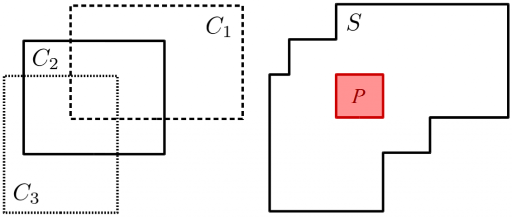
Well, first of all, let’s look at a crisp example (i.e., a simple star-shaped set that is not fuzzy), for example the one in Figure 1. How can we compute the size of the overall set S? The answer is quite simple: Compute the size of each of the three cuboids (by multiplying their width with their height) and use the inclusion-exclusion formula:

If we simply add the sizes of the three cuboids, we will count certain areas multiple times, namely the areas where two of the cuboids intersect. Therefore, we need to subtract the size of these areas from our result. By doing so, we however subtract a bit too much (namely, the region where all three cuboids intersect), so we need to add that again. Note that this inclusion-exclusion formula can easily be extended to more than 3 cuboids.
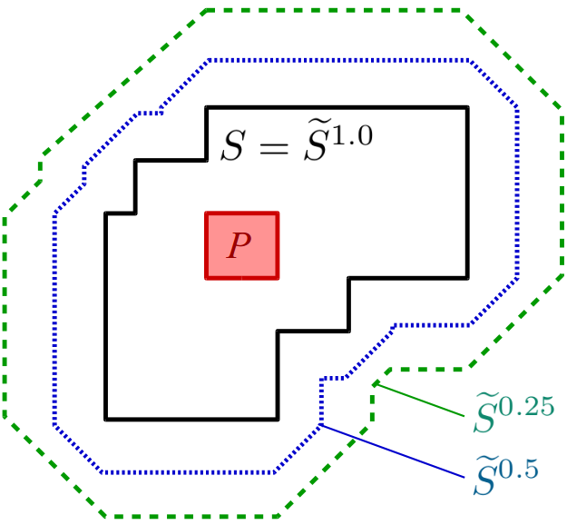
So computing the size of a non-fuzzy simple star-shaped set is actually not that complicated. But what about fuzzy simple star-shaped sets like the one in Figure 2? What is the size of this set?

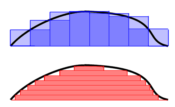
When dealing with fuzzy sets, one typically defines their size to be the area under their membership function, i.e., the integral of the membership function. There are two ways of computing this integral: The Riemann integral (which is what is typically taught in school) basically sums up vertical slices of the area under the curve, whereas the Lebesgue integral basically sums up horizontal slices of the area under the curve. Both variants are illustrated in Figure 3.

If we use the Riemann integral, we thus need to sum up for each point in the conceptual space the membership of this point to our fuzzy concept. If we use the Lebesgue integral, we need for each possible membership value α (i.e., for each number between 0 and 1) add up the size of the respective α-cut of the fuzzy set. Remember that the α-cut is simply the set of all points with a membership of at least α. If you look at Figure 2, this means that for α = 1.0, we get exactly the set S, for α = 0.5, we get the region marked by the blue boundary, and for α = 0.25 the region within the green border.
In most practical cases, it doesn’t really matter which of the two types of integrals you use, because both will come up with the same result (after all, they try to compute the same thing). However, the mathematical proof layed out in my paper [1] becomes much easier if we use the Lebesgue integral, so we will focus on this approach. So what we need to do is to figure out how large each α-cut of a fuzzy concept is.
Because the membership of a point x to a fuzzy concept becomes smaller with increasing distance, we can think of each α-cut as being a so-called ε-neighborhood of the original crisp set S (i.e., the region of all points that have a distance of at most ε to S). The challenge we now face is that we need to describe the size of each α-cut in some mathematical way.

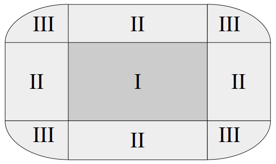
Figure 4 illustrates an α-cut for a single cuboid. The region labeled with “I” is the original cuboid itself and we already know how to compute its size: By multiplying its width with its height.
All the regions labeled with “II” can also be described as rectangles. The two regions to the left and to the right of the original cuboid have the same height as the cuboid itself. Their width depends on α (“How far can we walk away from the cuboid and still have a membership of at least α?”). I won’t go into details here about how to compute this width based on α, but it’s actually not too complicated. Analogously, the width of the bottom and top rectangles equals the width of the cuboid, and their height is again dependent on α.
All the regions labeled with “III” finally together form an ellipse. The width of this ellipse is equal to the combined width of the left and the right region labeled with “II”. Its height is equal to the combined height of the bottom and top region labeled with “II”. It’s also relatively straightforward to compute the area contained in an ellipse.
By adding together the sizes of the region labeled with “I”, “II”, and “III”, we thus get the overall size of the α-cut. By computing the Lebesgue integral over these sizes, we get the size of the overall fuzzy cuboid. Then, by using the inclusion-exclusion formula, we can combine the sizes of the individual fuzzy cuboids and get the size of the overall fuzzy concept.
Of course, things are a bit more complicated than what I’ve shown above – there are usually more than two dimensions involved and we need to deal with both the Manhattan distance as well as the Euclidean distance. The mathematical details about how to deal with all these things can be found in my SGAI paper [1] (preprint here) and its appendix (pdf here).
Although I presented a simplified version, I still hope that the discussion above gives you a rough intuitive understanding of what’s going on when we try to compute the size of a fuzzy concept. In one of my next posts, we will see which other operations on fuzzy concepts can be based on this notion of concept size. Stay tuned!
References
[1] Lucas Bechberger and Kai-Uwe Kühnberger: “Measuring Relations between Concepts in Conceptual Spaces” Thirty-seventh SGAI International Conference on Artificial Intelligence, Cambridge/UK, December 2017.
