
In the past, we have already talked about some machine learning models, including LTNs and β-VAE. Today, I would like to introduce the basic idea of linear support vector machines (SVMs) and how they can be useful for analyzing a conceptual space.
Hyperplanes for classification
A linear support vector machine tries to separate data points belonging to two classes by using a hyperplane. In a two-dimensional feature space, a hyperplane corresponds to a simple line. In general, a hyperplane can be expressed by the equation w · x + b = 0 where x corresponds to the feature vector, w is a weight vector and b is an intercept.
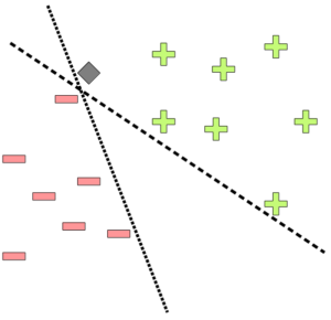
Figure 1 shows two example hyperplanes in a two-dimensional feature space which separate positive from negative examples. Unseen data points (such as the grey diamond) are classified by evaluating sign(w · x + b), i.e., by determining on which side of the hyperplane they lie. One can argue that while both hyperplanes in Figure 1 perfectly separate the two classes, they are probably not an optimal choice: Both lines lie alarmingly close to some of the training examples and might thus make wrong predictions.
For example, consider the data point represented by the grey diamond: It lies very close to one of the negative examples and not so close to the positive examples. Therefore, one would intuitively classify it as a negative. However, it lies on the “positive” side of both hyperplanes and is therefore classified as positive.
A maximum-margin hyperplane
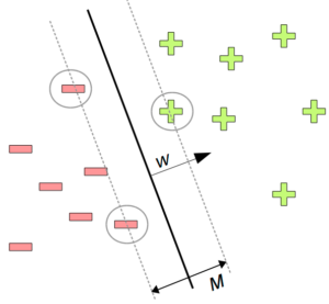
In order to avoid such misclassifications, a support vector machine tries to find a so-called “maximum margin” hyperplane, i.e., a decision boundary which has the largest possible distance to all example data points. This is illustrated in Figure 2, where the size of this margin is denoted by M. A support vector machine tries not only to separate the two classes from each other, but also to maximize M. This can be seen as a safety measure against future misclassifications. The name support vector machine stems from the observation that only certain data points are crucial for defining the decision boundary, namely the ones closest to the hyperplane (highlighted by circles in Figure 2).
I won’t describe how exactly an SVM finds the maximum margin hyperplane – if you’re interested in the mathematical details, you can take a look at the original publication [1]. An important point I would however like to highlight is that the weight vector w used in defining the hyperplane can be interpreted as the normal vector of the hyperplane. That is, w always is perpendicular to the decision boundary and therefore points from negative to positive examples. This is also illustrated in Figure 2 and will be important for the remainder of this blog post.
Using SVMs to analyze similarity spaces
As I have mentioned in an earlier post, the similarity spaces obtained by multidimensional scaling (MDS) usually don’t have interpretable coordinate axes. However, the conceptual spaces framework assumes that a conceputal space is spanned by such interpretable dimensions. In order to resolve this problem, Derrac and Schockaert [2] have used SVMs. I’ll now give you a rough idea about how that works.
Derrac and Schockaert have extracted a conceptual space for movies from a large collection of movie reviews. Basically, the similarity of two movies was defined as the similarity of their review texts. They then used MDS on these similarity ratings to extract a similarity space where each movie was represented as a point. I have already mentioned this conceptual space earlier, when I explained the setup for my LTN experiments. The problem is now that the dimensions of this similarity space are not necessarily meaningful. This means that if we know that two movies differ with respect to their third coordinate, we do not know how to interpret this difference, i.e., whether they differ with respect to humor, violence, or some other property. In most cases, such a difference in one coordinate of the MDS solution corresponds to a combination of multiple semantic features (e.g., being both funnier and less violent).
Even though such interpretable features do not necessarily coincide with the coordinate system of the similarity space, we can assume that they are still represented as directions in the space. In order to find such interpretable directions, Derrac and Schockaert have first created a list of candidate terms like “violent”, “funny” or “dancer” that appeared sufficiently often in the reviews. For each of these candidate terms, they divided the set of all movies into positive examples (i.e., movies whose reviews contained the candidate term) and negative examples (i.e., movies whose reviews did not contain the candidate term). They now applied a linear support vector machine to separate the positive from the negative examples. They then checked whether the SVM managed to find a maximum margin hyperplane that separated positive from negative examples sufficiently well. If this was the case, they took the weight vector w of this hyperplane as the direction representing the respective candidate term. Their reasoning was that w points from negative examples (i.e., movies not associated to this term) to positive examples (i.e., movies associated to this term).
This way, they were able to find directions for many terms such as the ones mentioned above. Thus, if we have two movies which differ in the “funny” direction, we can say that one of the movies is funnier than the other one. Derrac and Schockaert have done some more post-processing (e.g., grouping together similar directions such as “funny” and “hilarious”, and creating a new coordinate system based on the interpretable directions), which I will however skip here.
Outlook
The key insight you should remember is that the weight vector of a classification hyperplane points from negative to positive examples and that it can therefore be interpreted as a direction describing this classification difference spatially.
In one of my current studies, I have used the approach by Derrac and Schockaert to look for interpretable directions corresponding to meaningful psychological features in a similarity space of shapes. Today’s blog post can thus be seen as ground work for this analysis which will be the topic of a future blog post.
References
[1] Boser, B. E.; Guyon, I. M. & Vapnik, V. N.: “A Training Algorithm for Optimal Margin Classifiers” Proceedings of the Fifth Annual Workshop on Computational Learning Theory, Association for Computing Machinery, 1992, 144–152
[2] Derrac, J. & Schockaert, S.: “Inducing Semantic Relations from Conceptual Spaces: A Data-Driven Approach to Plausible Reasoning” Artificial Intelligence, Elsevier BV, 2015, 228, 66-94