
It’s about time for another blog post in my little “What is …?” series. Today I want to talk about a specific type of artificial neural network, namely convolutional neural networks (CNNs). CNNs are the predominant approach for classifying images and have already been implicitly used in my study on the NOUN data set as well as in the analysis of the Shape similarity ratings. With this blog post, I want to clarify the basic underlying structure of this type of neural networks.
Artificial Neural Networks in General
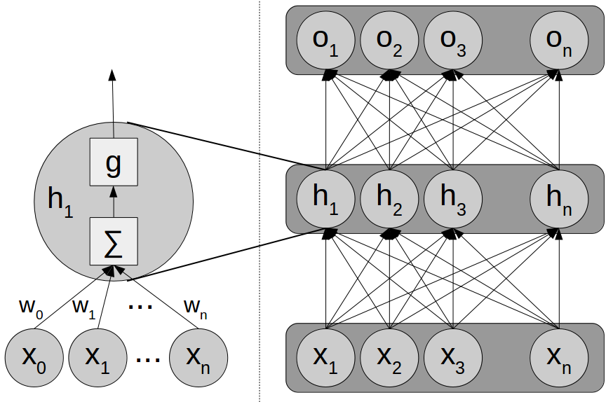
But first of all, a quick recap of artificial neural networks in general. These machine learning models consist of a large amount of interconnected individual units (also called “neurons”). Each unit computes a weighted sum of its inputs, puts this intermediate result through a nonlinear activation function (such as the sigmoid) and uses the resulting function value as its output (see the left part of Figure 1). Usually, these units are arranged in multiple layers and their connections are set up in such a way that each neuron in layer L receives input from all units in layer L-1 and broadcasts its output to all neurons in layer L+1 (see the right part of Figure 1). Training a neural network corresponds to estimating the weights on all of these connections in such a way, that the overall output of the network reflects the desired output as closely as possible. This type of network is often called “feed-forward network” or “multi-layer perceptron”.
Removing Connections and Sharing Weights
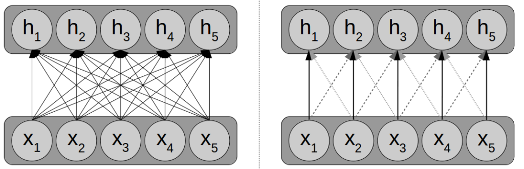
The main difference between convolutional neural networks and standard feed-forward networks lies in the way in which the connections between subsequent layers are set up. This is illustrated in Figure 2: While feed-forward networks typically use fully connected layers (left), convolutional neural networks remove a large part of these connections (right). More specifically, each neuron hi in the hidden layer receives input only from a small receptive field in the input layer – in our example, from the units xi-1, xi, and xi+1. All other connections (e.g., from x1 to h5) are removed from the network.
Moreover, the weights of the remaining connections are shared with each other – we enforce that the same weights are always used for connecting the inputs to the hidden unit. For example, the weight connecting x1 to h2 is identical to the weight connecting x3 to h4. This is indicated in Figure 2 by three different line styles for the three different weights.
As you can easily imagine, reducing the number of connections and enforcing weight sharing reduces the number of free parameters in the model quite drastically. In our example from Figure 2, we end up having to estimate only three weights for the convolutional layer, which is considerably less than the 25 weights needed in the fully connected case. This drastic reduction of parameters makes it possible to apply CNNs to high-dimensional inputs such as images.
Max Pooling
In addition to using weight sharing and small receptive fields, CNNs often employ a technique called “max pooling”. Essentially, this pooling step replaces each output of the hidden layer with the maximum over a small neighborhood of hidden units. Max pooling can be interpreted as a way of smoothing the output, but it also creates a certain invariance to small translations of the input. If the pooling result is not computed for every hidden unit, but for example only for every second hidden unit, this can also be used as a convenient way for reducing the dimensionality of the output.
Application to Image Data
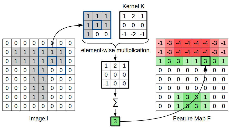
As mentioned in the beginning, CNNs have been very successful when being applied to images. Figure 3 illustrates how CNNs can be applied to a two-dimensional input (in this case, an image of the letter T). Essentially, the weights used for a convolutional layer can be interpreted as a so-called kernel. Since these weights are shared for all hidden neurons, the same kernel is applied to all input positions. This means, that for each position in the original image (highlighted in blue), we can compute an element-wise multiplication of the kernel with the respective receptive field, and sum over the individual results in order to obtain our weighted sum of inputs. This intermediate result is then put through a nonlinear activation function (left out in Figure 3 for the sake of simplicity) and gives the respecting output value at the current position.
Applying the kernel to all positions of the input and collecting the results gives us a so called feature map. In Figure 3, we have chosen a kernel which is useful for detecting horizontal lines. This can be easily seen by the values of the resulting feature map. Learning the weights of a convolutional layer thus corresponds to learning a transformation of the overall image which highlights certain aspects and which is based only on local information.
Useful Properties
Now why have CNNs been so successful on image data? The main reasons lie directly in the architectural changes we applied to standard feed-forward models:
Using only small receptive fields allows us to drastically reduce the number of parameters in the model and constrains us to using only local information. As Figure 3 illustrates, this is however still sufficient for extracting useful features (such as the presence or absence of horizontal lines).
Weight sharing further reduces the number of parameters and ensures that the same function is computed everywhere in the image – thus making it more likely to discover general transformations of the image instead of idiosyncratic sets of weights that are only useful in specific areas of the input.
The drastic reduction in the number of parameters makes it possible to process high-dimensional input (such as images with a high resolution). Moreover, it allows us do build deeper models with multiple convolutional layers stacked on top of each other. We can also use multiple kernels at the same time (e.g., in order to extract information about horizontal, vertical, and diagonal lines in an image, corresponding to three different feature maps).
The pooling function furthermore allows the output to be somewhat invariant to small translations and causes a certain “competition” between the hidden units. It can furthermore be used to reduce the size of the feature map, which is important if we want to go from high-resolution images to a low-dimensional representation that eventually leads to a binary classification decision.
And now?
Of course, what I have provided above is only a very rough sketch of convolutional neural networks. It leaves out many details and extensions, but should nevertheless suffice to convey a general intuition.
As I mentioned in the beginning, I have used the output of such a convolutional neural network both as a baseline for predicting human similarity ratings and as a feature space for a regression from images to points in psychological similarity spaces. In the next months, I’m going to apply CNNs again for such a regression task, this time with respect to the shape spaces mentioned above. So stay tuned!