
In my last blog post, I introduced my current research project: Learning to map raw input images into the shape space obtained from my prior study. Moreover, I talked a bit about the data set I used and the augmentation steps I took to increase the variety of inputs. Today, I want to share with you the network architecture which I plan to use in my experiments. So let’s get started.
The Overall Network Structure
First of all, let’s take a look at the big picture. My data set can be used for the three tasks of classification, mapping, and reconstruction. I therefore tried to come up with a general structure that incorporates these three tasks. Figure 1 shows the result of these considerations.
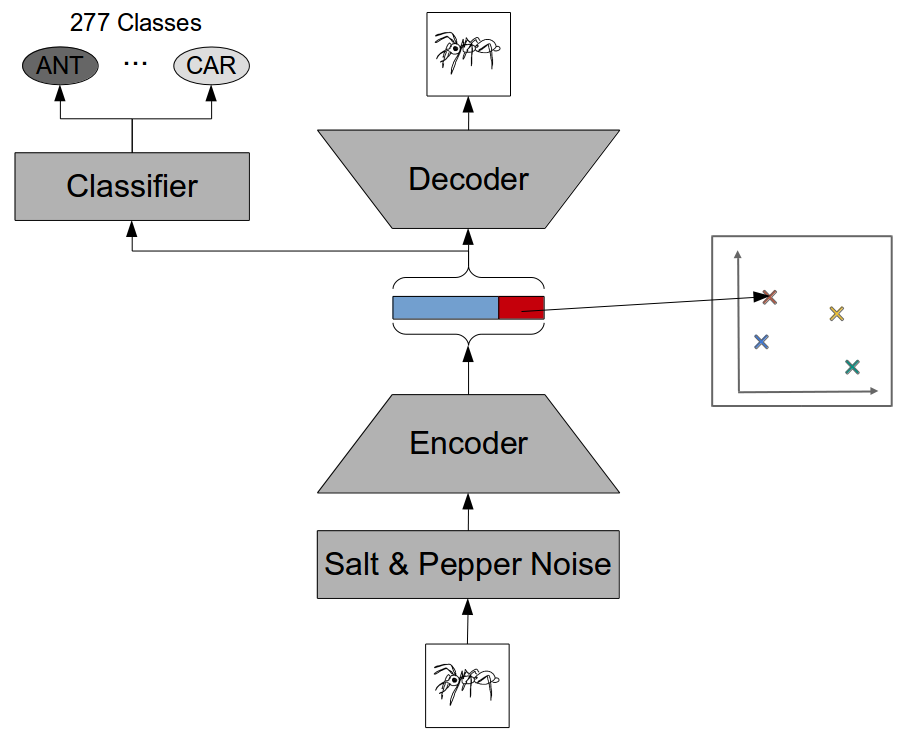
As you can see, we have several components. The input is first corrupted with some salt and pepper noise (i.e., by setting a random subset of pixels to white and black, respectively), before being fed into the encoder network. The job of this encoder network is to compress its high-dimensional input (128 x 128 = 16384 pixels) into a relatively low-dimensional representation (512 numbers or less). This “bottleneck” representation is then used as a basis for the three possible tasks:
For the classification task, we use a single fully connected layer with softmax activation to map the bottleneck representation to class probabilities of the 277 different classes of our data set. In Figure 1, this is represented by the classifier network.
For the mapping task, things are even simpler: We do not need any additional network, but we simply require that part of the bottleneck representation is identical to the target coordinates in our similarity space. For instance, if we consider a four-dimensional shape space, we simply take the last four entries of the bottleneck representation and interpret them as coordinates in this four-dimensional space. The mapping itself then needs to be learned by the encoder network.
For the reconstruction task, we feed the bottleneck representation though a decoder network, which tries to reconstruct the original input image from the compressed information. Since we try to reconstruct the original input and not the distorted one, our reconstruction objective corresponds to the one of a so-called denoising autoencoder.
As stated above, the classifier network is rather trivial. So let’s take a closer look at both the encoder and the decoder. We’ll start with the encoder.
Architecture of the Encoder
Since we’re dealing with image data, we use a convolutional neural network (CNN) for implementing the encoder. You can check out one of my recent blog posts to get a high-level idea of how CNNs work. More specifically, we’ll start by considering Sketch-a-Net [1], which is a variant of AlexNet [2] that explicitly targets sketches as inputs. Figure 2 compares the structure of AlexNet (the first CNN to achieve state of the art on ImageNet) to the one of Sketch-a-Net (the first CNN to achieve state of the art on the TU Berlin sketch data set).
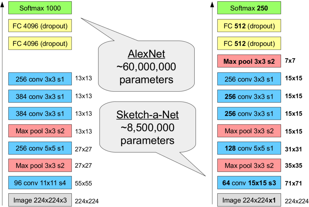
As we can see, both networks share the same overall structure, consisting of convolutional and max pooling layers and two fully connected layers at the end. While AlexNet comes with 60 million trainable parameters, Sketch-a-Net has only about 8.5 million weights. This has been achieved by reducing the number of convolution kernels, by using less neurons in the fully connected layers, and by introducing another max pool layer, which further reduces the representation size. Since sketches come without color and texture information, Sketch-a-Net uses larger kernels in the first convolutional layer to capture a larger receptive field.
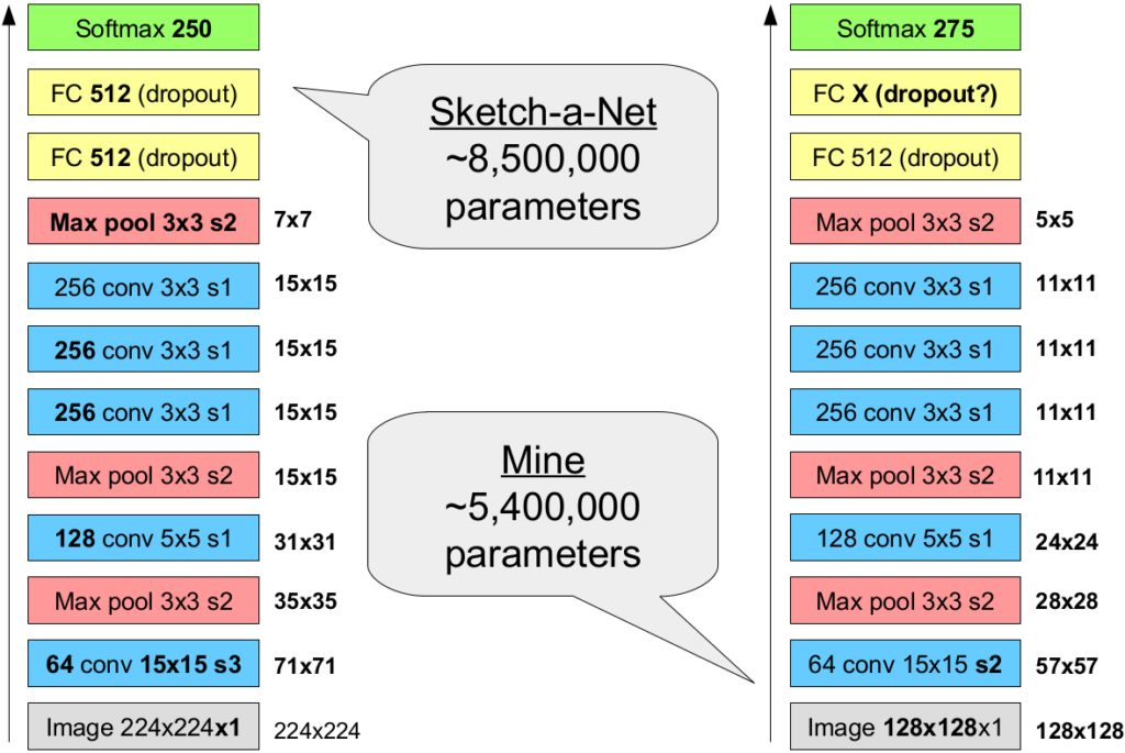
Figure 3 illustrates that my encoder network is a variant of Sketch-a-Net, which comes with again a smaller number of parameters. Since I am not so much interested in achieving state of the art results, I have decided to use a smaller image size of 128 by 128 pixels for the input, allowing me to use a stride of two (instead of three) in the first convolutional layer, while still ending up with a slightly smaller representation size and hence a smaller number of trainable parameters. Please note that the size of the final fully connected layer (which will serve as bottelneck layer in Figure 1) is treated as a hyperparameter – its default value will be 512, but I will try out different other variants as well.
Since both AlexNet and Sketch-a-Net have been successful, we can assume that also my encoder is likely to learn something useful. Of course, the performance of both AlexNet and Sketch-a-Net have been surpassed by more complex architectures. However, since I do not aim for state of the art performance anyways, keeping the network structure simple seems to be preferable. Having a smaller input size and fewer trainable parameters than the two networks from the literature should furthermore speed up the learning process, allowing me to conduct more experiments.
Architecture of the Decoder
The job of the decoder network is to map the low-dimensional bottleneck representation into the original high-dimensional image space. In order to do see how that works, we first have to introduce so-called “upconvolutional layers.”
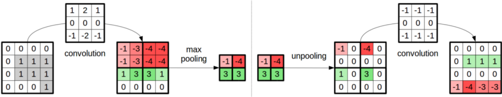
The left part of Figure 4 illustrates the typical processing step in a standard CNN: First, you apply a convolution to the given image patch, and then you use max-pooling to reduce the representation size. In order to approximately revert this process, an upconvolutional layer (shown in the right part of Figure 4) is based on an unpooling step (where you increase the representation size by filling in zeros between the input values) which is then followed by a regular convolution (which tries to fill in the gaps with more meaningful values). Although an upconvolutional layer is not really the inverse operation of “convolution + max pooling”, it still works reasonably well in practice.
So how is our decoder going to look like? Well, again I looked at the literature to find some suitable starting point. What I found is the work by Dosovitskiy and Brox [3], who used upconvolutional layers to reconstruct the original input from the high-level activation of AlexNet. Figure 5 illustrates their architecture in comparison to my decoder.
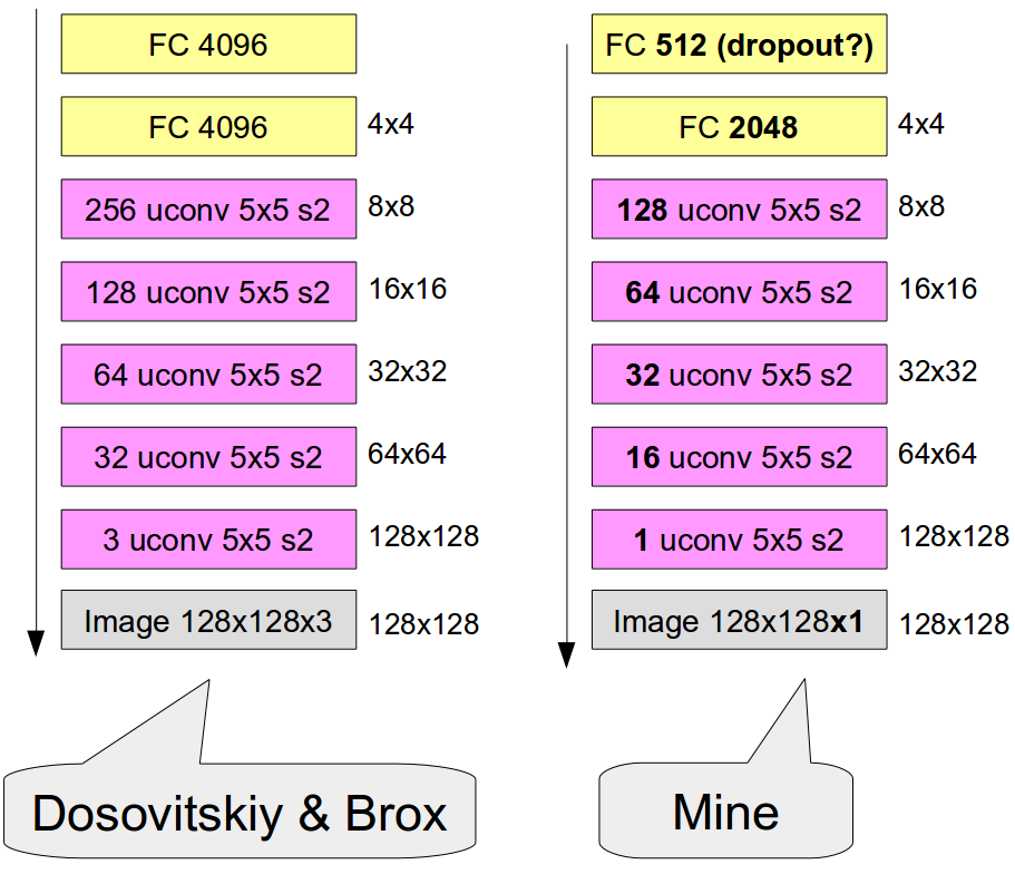
As one can see, both networks are quite similar in their structure: They have two fully connected layers, followed by multiple upconvolutional layers, and result in output images of size 128 x 128. Since the output in our case only contains greyscale information and is only based on black lines and white background, I have halved the number of convolutional kernels as well as the size of the second fully connected layer. For the first fully connected layer, I have furthermore chosen 512 units in order to mimic the first fully connected layer of the encoder. Again, since Dosovitskiy and Brox were able to achieve good results with their setup, I hope that it will also work reasonably well in my context.
What’s next?
Okay, so this has already been quite a lot of information. For today, I’ll leave it a that. Next time, I will write a bit about the overall experimental setup (i.e., how to train and evaluate the network) as well as the different experiments I plan to run. In subsequent posts, I will then share the results of these experiments as they come in.
References
[1] Yu, Q.; Yang, Y.; Liu, F.; Song, Y.-Z.; Xiang, T. & Hospedales, T. M. Sketch-a-Net: A Deep Neural Network that Beats Humans International Journal of Computer Vision, Springer, 2017, 122, 411-425
[2] Krizhevsky, A.; Sutskever, I. & Hinton, G. ImageNet Classification with Deep Convolutional Neural Networks Advances in Neural Information Processing Systems, Curran Associates, Inc., 2012, 25, 1097-1105
[3] Dosovitskiy, A. & Brox, T. Inverting Visual Representations With Convolutional Networks Proceedings of the IEEE Conference on Computer Vision and Pattern Recognition (CVPR), 2016