
Today, I would like to continue my little series about recent joint work with Margit Scheibel on a psychologically grounded similarity space for shapes. In my first post, I outlined the data set we worked with, and in my second post, we investigated how well the dissimilarity ratings are reflected by distances in the similarity spaces. Today, I’m going to use the categories from our data set to analyze whether conceptual regions are well-formed.
Our Expectations
Before we start our analysis, let us first define what exactly we expect to find based on the conceptual spaces framework. Please remember that the stimuli from our data set are grouped into twelve categories. Of these twelve categories, six are based on visual similarity while the remaining six contain visually variable items. Each of these categories can be interpreted as a concept in our framework. The visually coherent categories can be defined solely based on visual similarity, hence they should correspond to well-formed regions in shape space. The visually variable categories on the other hand cannot be defined only based on shape information, hence we don’t expect them to yield well-formed regions in shape space.
An important assumption of the conceptual spaces framework is that conceptual regions should be convex. Although I have challenged this assumption, my criticism targeted mainly the description of concepts that span multiple domains. For properties (which are defined only on a single domain), convexity may still apply. Since we are dealing here with a single domain, we thus assume that the categories of our data set can be represented by convex regions.
Conceptual regions do in general not overlap: Such an overlap only takes place in case of conceptual hierarchies (such as dog isa mammal) or for borderline items (e.g., a tomato which could be classified as both a vegetable or a fruit). As both cases do not apply to our data set, we can assume that there is no overlap between conceptual regions for visually coherent categories. Visually variable categories however contain items with quite different shape – they therefore might overlap with other regions.
Moreover, if each visually coherent category can be described based on visual similarity, then all of its items should be quite close to the category prototype in the shape space. For the visually variable categories, we can however not expect such a strong clustering. This means that we expect conceptual regions of visually coherent categories to be considerably smaller than the regions representing visually variable categories.
Overall, we may furthermore expect that the representational capability of the similarity space improves as more dimensions are added. Hence, we expect better results in higher-dimensional spaces.
Measuring Conceptual Overlap
So let’s start our analysis by investigating whether the conceptual regions of our categories overlap with each other. In order to quantify this notion of conceptual overlap, we first construct the convex hull for each category based on its items. For each of the categories, we then count how many “intruder” items from other categories lie within its convex hull. Figure 1 illustrates this idea.
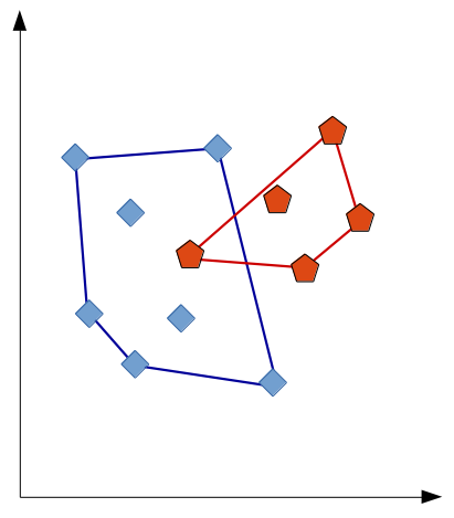
Here, the “blue” category has one intruder (as one point of the “red” category lies inside its convex hull), while the “red” category does not have any intruders. By aggregating the results across categories we can get the overall number of intruders (or violations of our assumptions). This summary information can be plotted as a function of the number of dimensions:
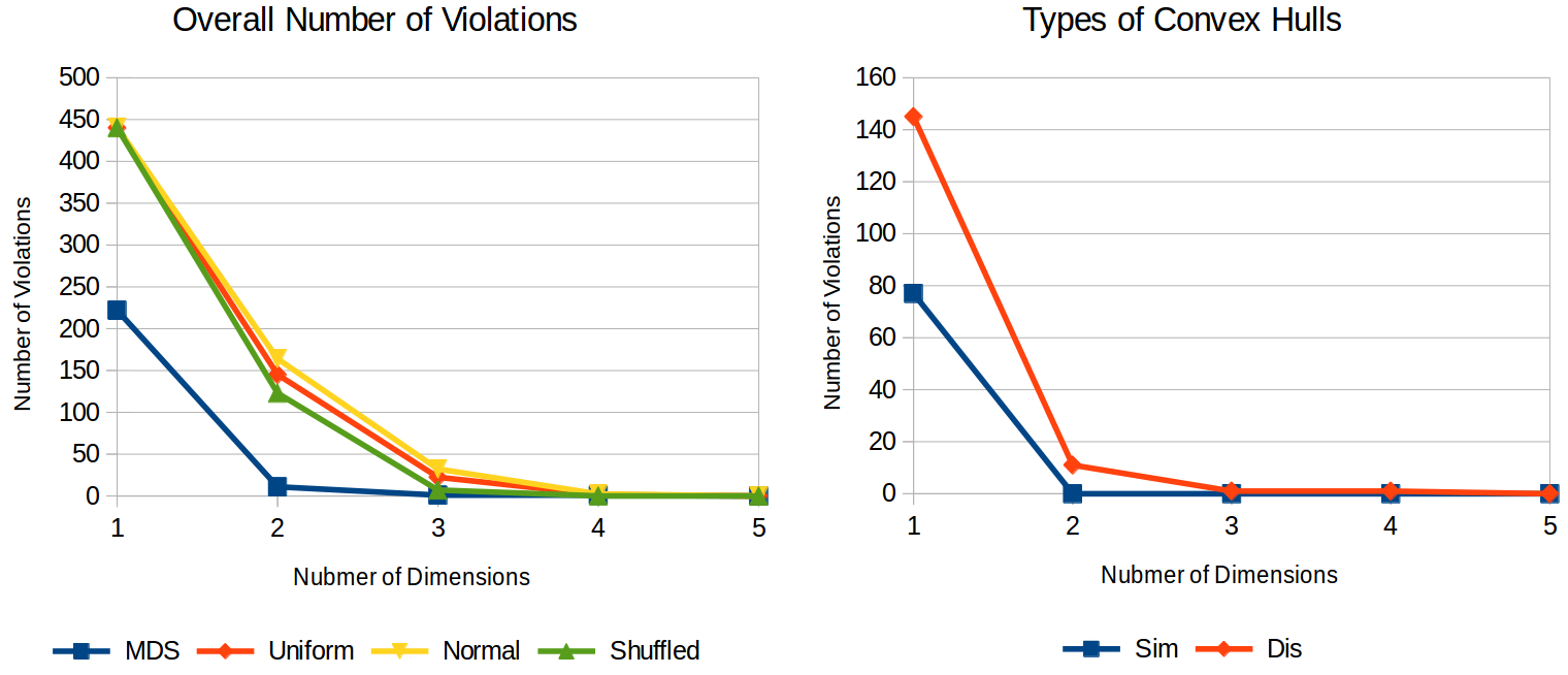
The left part of Figure 2 compares the overall number of violations that we found for our similarity spaces (labeled as MDS) to three baselines (where each item is associated with a randomly drawn point, based on either a uniform distribution, a normal distribution, or the shuffled set of points from the MDS solution). As we can see, the similarity spaces have a considerably lower number of violations than one would expect for randomly chosen points. However, even if we choose points at random, we don’t see any overlap in a five-dimensional space. This is probably based on the limited number of items per category (namely, 5). Since there is no difference between MDS and the baselines for high-dimensional spaces, we should probably not put too much weight on this information.
The right part of Figure 2 splits the number of violations according to the category type. Categories based on visual similarity have a smaller number of intruders than visually variable categories, which confirms our expectations: While visually coherent categories are well-formed in shape space, visually variable categories are not.
Measuring Conceptual Size
Okay, now let’s take a look at the size of the conceptual regions. In order to quantify this notion, we define the prototype of a category by computing the centroid of its members. The size of a category can then be measured as the average distance of its category members to this prototype. Again, we can aggregate across different categories in order to obtain more global information.
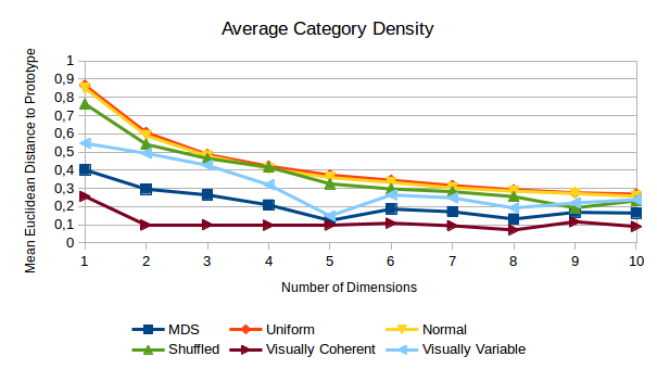
Figure 3 plots the average category size as a function of the number of dimensions. Which observations can we make? Well, first of all, the categories tend to be smaller than one would expect for randomly chosen points. Second of all, visually coherent categories are in general smaller than visually variable categories. Moreover, the size of the visually coherent categories stays pretty much constant from two dimensions onwards.
The average category size for the three baselines decreases with an increasing number of dimensions and so does the size of the visually variable categories. However, we can observe two weird bumps for the visually variable categories at five and eight dimensions. It’s still unclear to me where these bumps are coming from, even though I’ve spent quite some time investigating them. My best guess is that they are some random artifacts from the MDS algorithm, but their existence casts doubt on the reliability of this kind of analysis.
Conclusions
Overall, it seems that our expectations are fulfilled: Visually coherent categories are smaller than visually variable categories. Moreover, the convex regions of visually coherent categories contain only very few intruders – less than visually variable categories and certainly less than one would expect. It thus seems like the visually coherent categories can be interpreted as properties in the shape domain.
However, our analysis does not seem to be too reliable: On the one hand, number of intruders goes to zero anyways as soon as we have enough dimensions in the space. This can potentially be counteracted by considering more example members per category in future studies. On the other hand, we observed some weird effects for the size of visually variable categories that cannot be easily explained.
Therefore, while our findings with respect to conceptual regions do not contradict the conceptual spaces theory, they can only be seen as weak support. This concludes the second part of our analysis. Next time, we will finally look at the process of identifying interpretable directions in our shape spaces. Stay tuned!