
This post will be the last one in my mini-series “A Similarity Space for Shapes” about joint work with Margit Scheibel. So far, I have described the overall data set, the correlation between distances and dissimilarities, and the well-shapedness of conceptual regions. Today, I will finally take a look at interpretable directions in this similarity space.
Motivation
Remember from my first post in this mini-series that our data set contains ratings for each image with respect to three psychological features:
- FORM: Is the shape elongated or blob-like?
- LINES: Does the shape consist of straight or curved lines?
- ORIENTATION: Is the shape horizontally, diagonally, or vertically oriented?
Our hypothesis was that these three dimensions can be used as interpretable dimensions of the shape space. However, as we have seen when analyzing correlations, the space spanned by these three features is not better at predicting dissimilarities than a pixel-based comparison of the underlying images. This indicates that there seems to be more to shape similarity than captured by these three features. However, we might still be able to find directions in the similarity spaces obtained by MDS which reflect these three features. This is what we will discuss in the following.
The Procedure
In an earlier blog post, I have already introduced the basic idea behind linear support vector machines. Back then, I also referenced the work by Derrac and Schockaert [1] who used them for identifying interpretable directions in a similarity space. They defined a classification problems for each of their candidate features and then trained a linear SVM to separate the two classes (defined by presence and absence of the respective feature, respectively). If this separation was successful, they used the normal vector of the linear SVM’s hyperplane as the direction corresponding to the given candidate feature.
We essentially followed the same approach in our analysis: For each of the psychological features, we constructed a classification problem by ranking the images according to their feature value and taking the top and bottom 25% as positive and negative examples, respectively. We excluded the middle 50% in order to eliminate noise and to make the classification problem easier to solve. For each of the MDS-based similarity spaces, we then trained a linear SVM on this classification problem and measured the success by using Cohen’s kappa, which is essentially a normalized version of the classification accuracy that takes into account the probability of random guesses being correct.
The Results
Let us first take a look at Figure 1, which plots the classification performance for the three psychological features as a function of the dimensionality of the underlying similarity space.
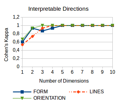
As we can see, a one-dimensional space is not sufficient for finding interpretable directions. However, already in a two-dimensional space, we are quite successful in identifying the features FORM and ORIENTATION. As soon as we add a third dimension, also the LINES feature can be reliably detected. From a five-dimensional space onwards, we reach perfect classification performance.
It thus seems that the distinction between the positive and negative examples for each feature is reflected by the spatial arrangement of the images in the similarity spaces. Already in a three-dimensional space, we quite successfully identify all three psychological features, confirming their status as being fundamental to shape perception.
In order to illustrate that the extracted directions are indeed meaningful, Figure 2 shows an illustration of our two-dimensional similarity space along with the three interpretable directions.

For both the FORM and the ORIENTATION feature, the resulting dimensions seem to reflect the differences between the positive and negative examples quite well. For the LINES feature, we can find counter-intuitive examples like the flowers mapping onto the “straight” end of the dimension, although their images contain more curved than straight lines. This poorer quality of the LINES direction is reflected by the lower values with respect to Cohen’s kappa as reported in Figure 1.
Outlook
This concludes our analysis of the shape space. As we have seen over the course of the last few blog posts, modeling shape perception with a conceptual space seems to be a promising approach: Distance is inversely related to similarity, we can find meaningful convex regions representing different categories, and the three features from the psychological literature on shape perception can be identified with directions in the similarity space. Thus, three core assumptions of the conceptual spaces framework are fulfilled.
Of course, the analysis we conducted was much more fine-grained than what has been described here in the blog. First presentations of our results at ICCS and CARLA (see my publications page for the abstracts and slides) were also limited to a relatively high level. We are currently preparing a journal article that gives a more detailed treatment of our results. If you are interested in how the analysis was exactly carried out and what the actual numbers are, please feel free to take a look at our code on GitHub.
Once we have wrapped up the analysis of the similarity spaces themselves, the next step for me will be to apply machine learning algorithms in order to learn a mapping from raw images into the similarity spaces. This will then hopefully be a nice follow-up on the results already reported on the NOUN data set.
References
[1] Derrac, J. & Schockaert, S.: “Inducing Semantic Relations from Conceptual Spaces: A Data-Driven Approach to Plausible Reasoning” Artificial Intelligence, Elsevier BV, 2015, 228, 66-94